20.1 Sampling distribution: Known proportion
Suppose a fair, six-sided die8 is rolled 25 times. What proportion of the rolls will produce an even number? That is, what will be the sample proportion of even numbers?
No-one knows exactly what will happen for any individual roll, so no-one knows what proportion will be even for any set of 25 rolls.
In addition, the proportion of the 25 rolls that will be even will not be the same for every set of 25 rolls. The sample proportion will vary: there is sampling variation.
Describing how the sample proportion varies from sample to sample is useful (Sect. 15.4.2).
To do this, statistical theory could be used… or thousands of repetitions of a set of 25 rolls could be performed… or a computer could simulate many sets of 25 rolls.
Let’s simulate rolling a die 25 times, using just 10 sets of 25 rolls; see the animation below.
The proportion of rolls that is even varies from set to set. For these 10 sets of \(n=25\) rolls, the percentage of even rolls ranged from \(\hat{p}=0.32\) even rolls to \(\hat{p}=0.60\) even rolls.
The sample proportion of even rolls would be expected to vary around \(p=0.5\), since three of the six faces of the die are even numbers (the population proportion), using the classical approach to probability.
Of course, the sample proportion could be very small or very high by chance, but we wouldn’t expect to see that very often.
In this example, the population proportion of even rolls is known to be \(p=0.5\). Each set of \(n=25\) rolls is a sample of all possible sets of \(n=25\) rolls, and the sample proportion of even rolls is denoted by \(\hat{p}\).
For any set of 25 rolls, the value of \(\hat{p}\) will be unknown until we roll the die. The proportion of even rolls is likely to vary from sample to sample; that is, the sample proportions exhibit sampling variation, and the amount of sampling variation is quantified using a standard error.
Suppose a fair die was rolled 25 times, and this was repeated thousands of times (not just 10 sets times, as in the animation above), and the proportion of even rolls was recorded for every set of 25 rolls.
These thousands of sample proportions \(\hat{p}\), one from every set of 25 rolls, could be graphed using a histogram; see the animation below.
The shape of the histogram is roughly a normal distribution. This is no accident: statistical theory says this will happen (when certain conditions are met: see Sect. 20.6).
The possible values of the sample proportion \(\hat{p}\) have a sampling distribution which is roughly a normal distribution; the mean and standard deviation of the normal distribution the animation above can even be determined. The possible values of the sample proportion \(\hat{p}\) will have a sampling distribution, described by:
- an approximate normal distribution;
- centred around a mean of \(p=0.5\);
- with a standard deviation of 0.1 (where this number comes from will be revealed soon).
This distribution is called a sampling distribution, as discussed in Sect. 18.1. The standard deviation of the sampling distribution is called a standard error, since it measures how much a sample statistic (in this case, a sample proportion \(\hat{p}\)) varies from sample to sample.
Since the variation in the sample proportions can be described, a picture of this normal distribution can be drawn (Fig. 20.1). We still don’t know exactly what we’ll find next roll… but we have some idea of how the sample proportion is likely to vary in sets of 25 rolls.
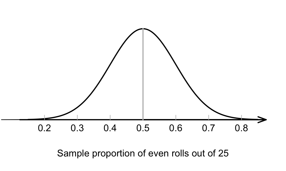
FIGURE 20.1: The normal distribution, showing how the proportion of even rolls varies when a die is rolled 25 times
The value of \(p\) (the population proportion: the proportion of even numbers on the die) remains the same, but the value of \(\hat{p}\) (the sample proportion: the proportion of even numbers in the sample of 25 rolls) is not the same in every set of 25 rolls. That is, \(\hat{p}\) varies, and exhibits sampling variation. The variation in \(\hat{p}\) from sample to sample is measured by the standard error of the sample proportion, written as \(\text{s.e.}(\hat{p})\).
In general, the standard error for a sample proportion when \(p\) is known is given by
\[\begin{equation} \text{s.e.}(\hat{p}) = \sqrt{\frac{p \times (1-p)}{n}}, \tag{20.1} \end{equation}\] where \(n\) is the number of rolls, and \(p\) is the population proportion. For this example, there are \(n = 25\) rolls of a die, and the population proportion of even rolls is \(p=0.5\). Then, the standard error of the sample proportion is
\[\begin{equation} \text{s.e.} (\hat{p}) = \sqrt{\frac{0.5 \times (1-0.5)}{25}} = 0.1. \tag{20.2} \end{equation}\]
This standard deviation is the standard deviation of the normal distribution in Fig. 20.1.
Recall that the the standard error is just a special standard deviation, that measures how much a sample estimate is likely to vary from sample to sample. In that sense, the standard error of the proportion measures how precisely \(\hat{p}\) estimates the population proportion \(p\).
Almost always, the value of \(p\) is unknown, so when \(\text{s.e.}(\hat{p})\) is computed, the value of \(p\) can’t be used. Instead, the best available estimate of \(p\) is used, which is \(\hat{p}\). This situation is studied from Sect. 20.3 onwards.
Definition 20.1 (Sampling distribution of a sample proportion when \(p\) is known) When the value of \(p\) is known, the sampling distribution of the sample proportion is described by
- an approximate normal distribution,
- centred around a mean of \(p\),
- with a standard deviation (called the standard error of \(\hat{p}\)) of
\[ \text{s.e.}(\hat{p}) = \sqrt{\frac{ p \times (1-p)}{n}}, \]
when certain conditions are met, where \(n\) is the size of the sample, and \(p\) is the population proportion.
In general, the approximation gets better as the sample size gets larger.Think 20.1 (Values for \(\hat{p}\)) From the die example, the values of \(\hat{p}\) will vary
- with an approximate normal distribution;
- centred around \(p=0.5\); and
- with a standard error of approximately \(\text{s.e.}({\hat{p}}) = 0.1\).
Note the language: two dice, but one die. Dice is plural.↩︎