20.2 Sampling intervals: Known proportion
The possible values of the sample proportions \(\hat{p}\) can be described by an approximate normal distribution, as just discussed. This enables the 68–95–99.7 rule to be applied; for example, about 68% of the time with sets of 25 rolls, the sample proportion of even rolls will be between \(0.5\) give-or-take one standard deviation (that is, give-or-take 0.1). So, about 68% of the time, the proportion of even rolls in a set of 25 rolls will be between:
- \(0.5 - 0.1 = 0.4\) and
- \(0.5 + 0.1 = 0.6\).
Similarly, about 95% of the time, the proportion of even rolls will be between \(0.5\) give-or-take two standard deviations, or between:
- \(0.5 - (2\times0.1) = 0.3\) and
- \(0.5 + (2\times0.1) = 0.7\).
This interval tell us what values of \(\hat{p}\) are likely to be observed in samples of size 25. Most of the time (i.e., approximately 95% of the time), the value of \(\hat{p}\) is expected to be between 0.30 and 0.70. (For instance, in the animation above, all ten sets of 25 rolls (or 100%) had a sample proportion betweeen 0.30 and 0.70.)
More formally, the sample proportion \(\hat{p}\) is likely to lie within the interval
\[ p \pm (\text{multiplier} \times \text{s.e.}(\hat{p})), \] where \(\text{s.e.}(\hat{p})\) is the standard error of the sample proportion (calculated using Eq. (20.1)). The symbol ‘\(\pm\)’ means ‘plus or minus,’ or ‘give-or-take.’
The multiplier depends on how confident we wish to be that the interval contains the value of \(\hat{p}\).
For a 95% interval—the most common level of confidence—the multiplier is approximately 2, based on the 68–95–99.7 rule: Approximately 95% of observations are within two standard deviations of the value of \(p\) (the mean of the normal distribution in Fig. 20.1).
That is, the approximate 95% interval is:
\[ p \pm (2 \times \text{s.e.}(\hat{p}) ). \] For a 90% interval, either tables or a computer would be used to find the correct multiplier, since the 68–95–99.7 rule isn’t helpful.
In practice, 95% intervals are the most common, and we’ll use a multiplier of \(2\) to find an approximate 95% interval when computing the interval without using software. Software can be used for any other percentage interval (or for an exact 95% interval).
In general, higher confidence means wider intervals (Fig. 20.2), since wider intervals are needed to be more certain that the interval contains \(\hat{p}\).
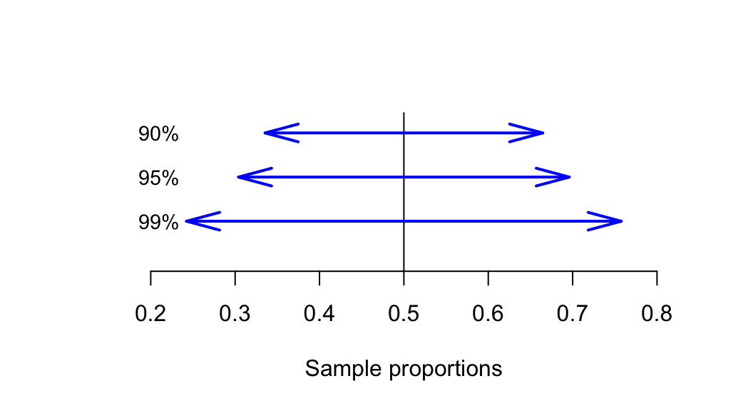
FIGURE 20.2: To have greater confidence that the interval will include the sample proportion, the interval needs to be wider