29.3 Sampling distribution: Expectation

Initially, assume that \(\mu_d = 0\). However, the sample mean energy saving will vary depending on which sample is randomly obtained, even if the mean saving in the population is zero: the sample mean energy saving has sampling variation and hence a standard error. The sampling distribution of \(\bar{d}\) can be described, which describes what values of the statistic might be expected in the sample if the \(\mu_d=0\).

Answering the RQ requires data. The data should be summarised numerically (using your calculator or software, such as jamovi (Fig. 29.1) or SPSS (Fig. 29.2)), and graphically (Fig. 23.1).

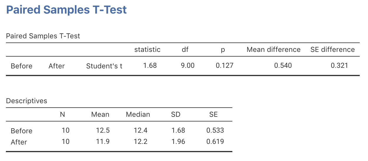
FIGURE 29.1: jamovi output for the insulation data

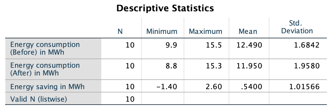
FIGURE 29.2: SPSS output for the insulation data

The sample mean difference is \(\bar{d}=0.5400\)… but this value of \(\bar{d}\) will vary from sample to sample even if \(\mu_d=0\). The amount of variation in \(\bar{d}\) is quantified using the standard error. More precisely, the possible values of the sample mean differences can, under certain conditions, described using

an approximate normal distribution; with
a mean of \(\mu_d = 0\) (taken from \(H_0\)); and
a standard deviation (called the standard error) of \(\text{s.e.}(\bar{d}) = s_d/\sqrt{n} = 0.3212\), where \(s_d\) is the standard deviation of the differences.

This describes what can be expected from the possible values of \(\bar{d}\) (Fig. 29.3), just through sampling variation (chance) if \(\mu_d=0\).

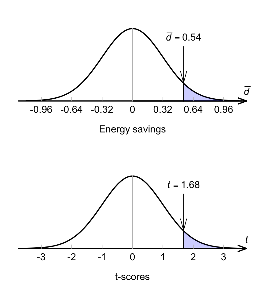
FIGURE 29.3: The sampling distribution of sample means, if the energy saving in the population really was zero