31.4 The test statistic: Observations
The decision-making process compares what is expected from the sample statistic if the null hypothesis about the parameter is true (Table 31.3) to what is observe in the sample (Table 31.1). Previously, when the summary statistics were means, \(t\)-tests were used. However, these data are not summarised by means, and a different test statistic is used.
Rather than using a \(t\)-score as the test-statistic, the test-statistic here is a ‘chi-squared’ statistic, written \(\chi^2\). A \(\chi^2\) statistic measures the overall size of the differences between the expected counts and observed counts, over the entire table.
The Greek letter \(\chi\) is pronounced ‘ki,’ as in kite.
The test statistic \(\chi^2\) is pronounced as ‘chi-squared.’From the software
(jamovi: Fig. 31.1;
SPSS: Fig. 31.2),
\(\chi^2=6.934\).
In a \(2\times 2\) table of counts
(when the ‘degrees of freedom,’ or df, is equal to 1,
as shown in the computer output),
the square root of the \(\chi^2\) value is
approximately equivalent to a \(z\)-score.
So here,
the equivalent \(z\)-score is about \(\sqrt{6.934} = 2.63\),
which is fairly large:
a small \(P\)-value is expected.
More generally, for two-way tables of any size,
\[ \sqrt{\frac{\chi^2}{\text{df}}} \] is like a \(z\)-score, where df is the ‘degrees of freedom’ (related to the size of the table15), as shown in the software output. This allows a \(P\)-value to be estimated using the 68–95–99.7 rule from the value of the \(\chi^2\) statistic.
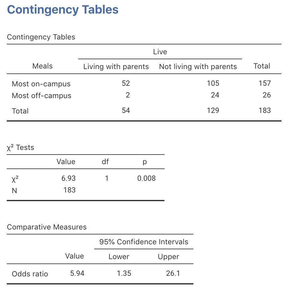
FIGURE 31.1: The jamovi output for computing a CI and conducting a test
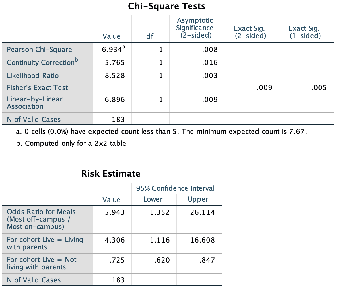
FIGURE 31.2: The SPSS output for computing a CI and conducting a test
df in the software output),
the value of
\[
\sqrt{\frac{\chi^2}{\text{df}}}
\]
is like a \(z\)-score.
This allows the \(P\)-value to be estimated using the
68–95–99.7 rule.
For those who want to know: the degrees of freedom in a two-way table is the number of rows of data minus one, times the number of columns of data minus one. So, for a two-way table, the degrees of freedom is \((2-1) \times (2-1) = 1\).↩︎