31.10 Example: Kerbside dumping

A study of dumping households goods on the kerbside in Brisbane (Comerford et al. 2018) asked people about their opinions on the dumping. All participants were from Brisbane suburbs where a high level of kerbside dumping occurred.
The data are summarised in Table 31.9. Notice that this is a \(2\times 3\) table of counts, so it is more difficult to define a parameter.
| Acceptable | Not acceptable | Conditionally acceptable | |
|---|---|---|---|
| Reuseable | 22 | 18 | 15 |
| Non-reuseable | 6 | 36 | 1 |
The software output is shown in Fig. 31.9 (for jamovi), and Fig. 31.10 (for SPSS); a graphical summary in Fig. 31.11.
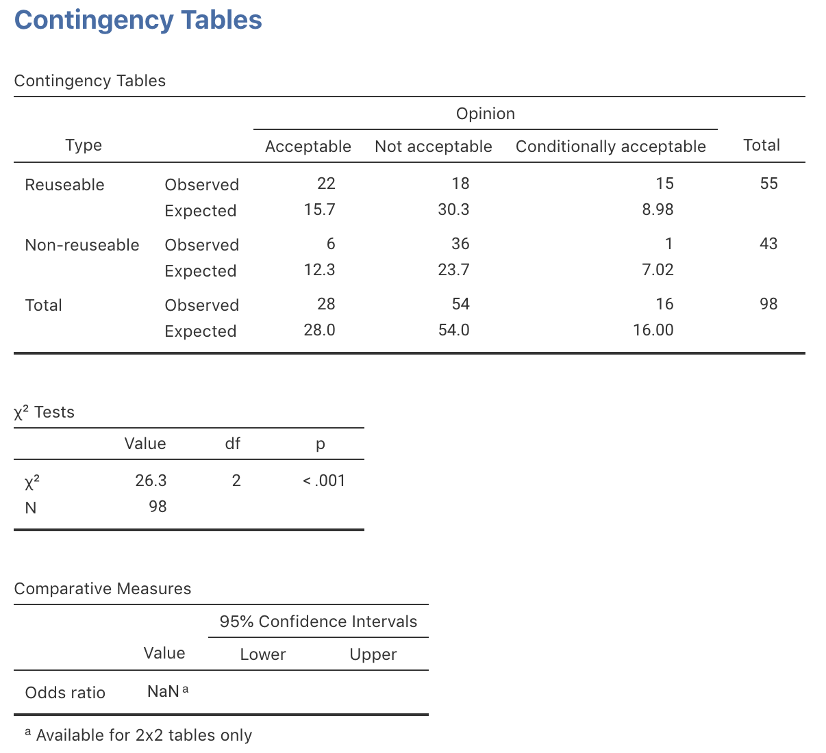
FIGURE 31.9: jamovi output for the kerbside-dumping data
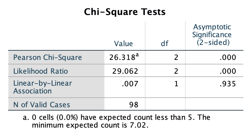
FIGURE 31.10: SPSS output for the kerbside-dumping data
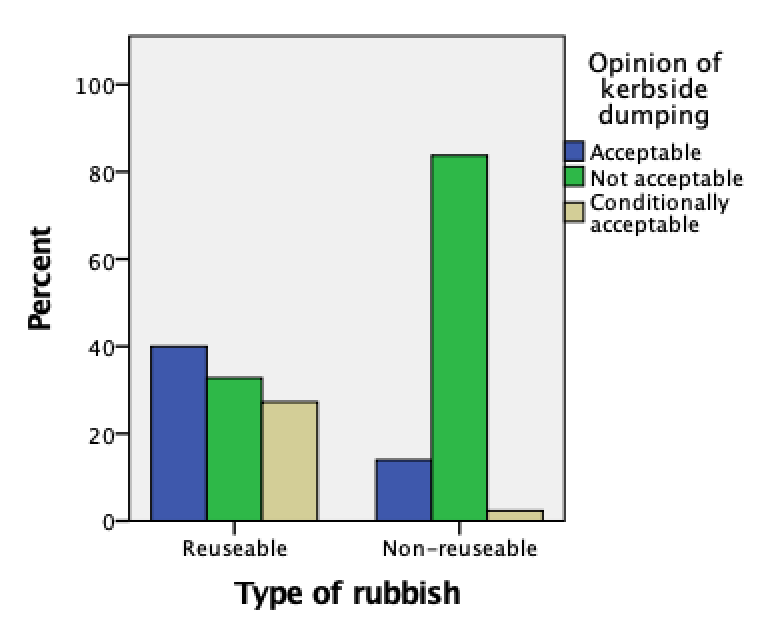
FIGURE 31.11: A side-by-side bar chart for the kerbside-dumping data
Most of the numerical summary must be produced manually (Table 31.10), since software only produces odds ratios for \(2\times 2\) tables.
| Odds | Odds ratio | Percentage | Sample size | |
|---|---|---|---|---|
| Acceptable: | 3.667 | (Reference) | 78.6% | 28 |
| Not acceptable: | 0.5 | 0.136 | 33.3% | 54 |
| Conditionally acceptable: | 15 | 4.09 | 93.4% | 16 |
In Table 31.10, the odds are that the given opinion refers to Reusable goods. Here are some of the details of these calculations:
- For Acceptable goods: the odds that these are reusable goods is \(22/6 = 3.667\).
- For Not acceptable goods: the odds that these are reusable goods is \(18/36 = 0.5\).
- For Conditionally acceptable goods: the odds that these are reusable goods is \(15/1 = 15\).
Then the odds ratios can be computed:
- Comparing the odds of Not acceptable to Acceptable: \(0.5/3.667 = 0.136\).
- Comparing the odds of Conditionally acceptable to Acceptable: \(15/3.667 = 4.09\).
Note that Table 31.10 has three groups to compare, so three odds calculations. However, the summary has \(3 - 1 = 2\) odds ratios, since odds ratios compare two odds. The level to which the other two are compared is called the Reference level. In Table 31.10, the reference level is ‘Acceptable.’
(In a \(2\times 2\) table, with two groups to compare, the summary has only \(2 - 1 = 1\) odds ratio.)
The hypotheses can be expressed in many ways (in terms of odds, odds ratio, or percentages), but perhaps the easiest approach with two-way tables larger than \(2\times 2\) is worded in terms of relationships or associations between the two variables:
- \(H_0\): There is no association between the type of rubbish and the opinion of kerbside duming.
- \(H_1\): There is an association between the type of rubbish and the opinion of kerbside duming.
From the software output, the \(\chi^2\)-value is 26.318 and the degrees of freedom is two, so this \(\chi^2\) value is approximately equivalent to a \(z\)-score of
\[ \sqrt{\frac{26.318}{2}} = 3.63. \] This is a large \(z\)-score so, using the 68–95–99.7 rule, a very small \(P\)-value is expected; indeed, the software output reports \(P<0.001\). This suggests very strong evidence in the sample that opinions are not the same for reuseable and non-reuseable rubbish.
The conclusion could be written as
The sample provides very strong evidence (\(\chi^2=26.318\); \(\text{df}=2\)) that there is a relationship in the population between opinions about kerbside dumping and the type of rubbish.
While sample summary information could be added, the conclusion statements then become cumbersome. Instead, pointing readers to the numerical summary (Table 31.10) is probably better. Furthermore, CIs are not reported since the software does not produce CIs for tables larger than \(2\times 2\).
All expected values all exceed 5 (as in the jamovi (Fig. 31.9) and SPSS output (Fig. 31.10)), even though one observed count is less than five. The results are statistically valid.