27.6 Making decisions with \(P\)-values
\(P\)-values tells us the likelihood of observing the sample statistic (or something more extreme), based on the assumption about the population parameter being true. In this context, the \(P\)-value tells us the likelihood of observing the value of \(\bar{x}\) (or something more extreme), just through sampling variation (chance) if \(\mu=37\). The \(P\)-value is a probability, albeit a probability of something quite specific, so it is a value between 0 and 1. Then:
‘Big’ \(P\)-values mean that the sample statistic (i.e., \(\bar{x}\)) could reasonably have occurred through sampling variation, if the assumption about the parameter (stated in \(H_0\)) was true (Fig. 27.7, top panel): The data do not contradict the assumption (\(H_0\)).
‘Small’ \(P\)-values mean that the sample statistic (i.e., \(\bar{x}\)) is unlikely to have occurred through sampling variation, if the assumption about the parameter (stated in \(H_0\)) was true: (Fig. 27.7, bottom panel): The data contradict the assumption.
What is meant by ‘small’ and ‘big?’ It is arbitrary: no definitive rules exist. Commonly, a \(P\)-value smaller than 1% (that is, smaller than 0.01) is usually considered ‘small,’ and a \(P\)-value larger than 10% (that is, larger than 0.10) is usually considered ‘big.’ Between the values of 1% and 10% is often a ‘grey area.’
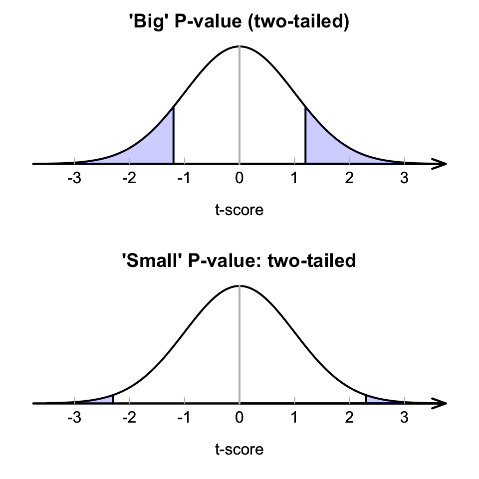
FIGURE 27.7: A picture of large (top) and small (bottom) \(P\)-value situations
Traditionally, a \(P\)-value is ‘small’ if it is less than 5% (less than 0.05), and ‘big’ if greater than 5% (greater than 0.05). However, again this is arbitrary, and binary decision making (either big or small) is unreasonable. More reasonably, \(P\)-values should be interpreted as providing varying strength of evidence in support of the alternative hypothesis \(H_1\) (Table 27.1. These are not definitive, but are only guidelines. Of course, conclusions should be written in the context of the problem.
| If the \(P\)-value is… | Write the conclusion as… |
|---|---|
| Larger than 0.10 | Insufficient evidence to support \(H_1\) |
| Between 0.05 and 0.10 | Slight evidence to support \(H_1\) |
| Between 0.01 and 0.05 | Moderate evidence to support \(H_1\) |
| Between 0.001 and 0.01 | Strong evidence to support \(H_1\) |
| Smaller than 0.001 | Very strong evidence to support \(H_1\) |
For one-tailed tests, the \(P\)-value is half the value of the two-tailed \(P\)-value.
SPSS always produces two-tailed \(P\)-values, usually calls them ‘Significance values,’ and labels them asSig.,
and sometimes explicitly notes that they are two-tailed.
For the body-temperature data then, where \(P<0.001\), the \(P\)-value is very small, so there is very strong evidence that the population mean body temperature is not \(37.0^\circ\text{C}\).