27.13 Exercises
Selected answers are available in Sect. D.25.
Exercise 27.1 The recommended daily energy intake for women is 7725kJ (for a particular cohort, in a particular country; Altman (1991)). The daily energy intake for 11 women was measured to see if this is being adhered to. The RQ is
For this group of women, is the population mean daily energy intake 7725kJ?
The data collected are shown in Table 27.3.
- Write the hypotheses for answering this RQ.
- Use the jamovi output (Fig. 27.11), write down the value of \(\bar{x}\) and \(\text{s.e.}(\bar{x})\).
- Using this output, write down the \(t\)-value and the \(P\)-value.
- Write a suitable conclusion.
- Is the test statistically valid?
- Sketch the sampling distribution of \(\bar{x}\).
| 5260 | 5640 | 6390 | 6515 | 7515 | 8770 |
| 5470 | 6180 | 7515 | 6805 | 8230 |
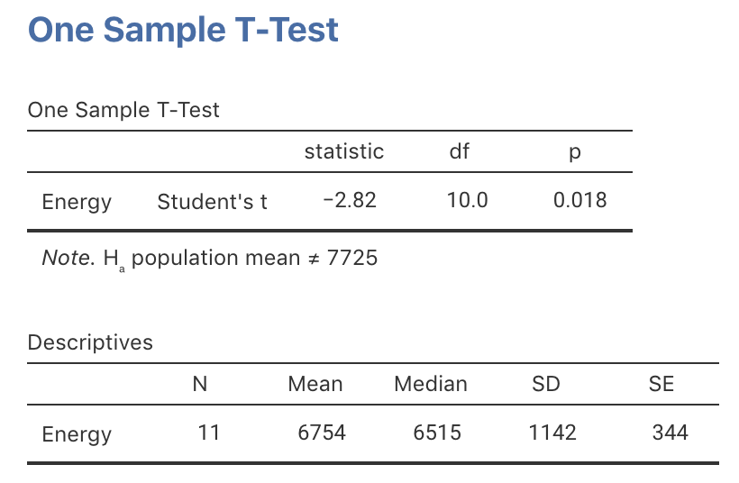
FIGURE 27.11: jamovi output for the energy-intake data
Exercise 27.2 Most dental associations11 recommend brushing teeth for two minutes. A study (Macgregor and Rugg-Gunn 1979) of the brushing time for 85 uninstructed school children from England (11 to 13 years old) found the mean brushing time was 60.3 seconds, with a standard deviation of 23.8 seconds.
- Is there evidence that the mean brushing time for schoolchildren from England is two minutes (as recommended)?
- Sketch the sampling distribution of the sample mean.
Exercise 27.3 A study (Greenlee et al. 2018) of human-automation interaction with automated vehicles aimed to
… determine whether monitoring the roadway for hazards during automated driving results in a vigilance decrement.
— Greenlee et al. (2018), p. 465
(A ‘decrement’ is a reduction.) That is, they were interested in whether the average mental demand of ‘drivers’ of automated vehicles was higher than the average mental demand for ordinary tasks.
In the study, the \(n=22\) participants ‘drove,’ in a simulator, an automated vehicle for 40 minutes. While driving, the drivers monitored the road for hazards. The researchers assessed the ‘mental demand’ placed on these drivers, where scores of 50 over ‘typically indicate substantial levels of workload’ (p. 471). For the sample, the mean score was 84.00 with a standard deviation of 22.05.
Is there evidence of a ‘substantial workload’ associated with monitoring roadways while ‘driving’ automated vehicles?Exercise 27.4 A study explored the quality of life of patients receiving cavopulmonary shunts (Steele et al. 2016). ‘Quality of life’ was assessed using a 36-question health survey, where the scale is standardised so that the mean of the general population is 50.
For the 14 patients in the study, the sample mean for the ‘Physical component’ of the survey was 47.2 (with a standard deviation of 8.2). The sample mean for the ‘Mental component’ of the survey was 52.7 (with a standard deviation of 5.6).
Is there evidence that the patients are different, on average, to the general population on the basis of the results?
FIGURE 27.12: jamovi output for the Cherry Ripes data
Exercise 27.6 A study of paramedics (Williams and Boyle 2007) asked participants (\(n=199\)) to estimate the amount of blood on four different surfaces. When the actual amount of blood spilt on concrete was 1000 ml, the mean guess was 846.4 ml (with a standard deviation of 651.1 ml).
Is there evidence that the mean guess really is 1000 ml (the true amount)? Is this test likely to be valid?| High level (Inst. 1) | Mid level (Inst. 1) | High level (Inst. 2) | Mid level (Inst. 2) | |
|---|---|---|---|---|
| Mean of data | 64.31 | 19.240 | 64.970 | 19.400 |
| Std. dev. of data | 1.70 | 0.588 | 1.029 | 0.413 |
| Pre-determined target | 64.22 | 19.010 | 65.050 | 19.450 |
References
Such as the American Dental Association and the Australian Dental Association.↩︎