17.8 Examples using \(z\)-scores
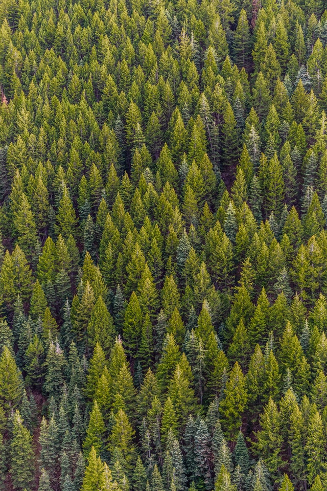
Example 17.7 (Normal distributions) Aedo-Ortiz et al. (1997) simulated mechanized forest harvesting systems (Devore and Berk 2007).
As part of their study, they assumed that the specific trees in their study would vary in diameter, with
- a normal distribution; with
- a mean of \(\mu=8.8\) inches; and
- a standard deviation of \(\sigma=2.7\) inches.
Follow the steps identified earlier:
- Draw a normal curve, and mark on 6 inches (Fig. 17.7, top panel).
- Shade the region corresponding to ‘greater than 6 inches’ (Fig. 17.7, bottom panel).
- Compute the \(z\)-score using Eq. (17.1). Here, \(x=6\), \(\mu=8.8\), \(\sigma=2.7\), so \(\displaystyle z = (6 - 8.8)/2.7 = -2.8/2.7 = -1.04\) to two decimal places.
- Use tables: The probability of a tree diameter shorter than 6 inches is \(0.1492\). (The tables always give area less than the value of \(z\) that is looked up.)
- Compute the answer: Since the total area under the normal distribution is one, the probability of a tree diameter greater than 6 inches is \(1 - 0.1492 = 0.8508\), or about 85%.
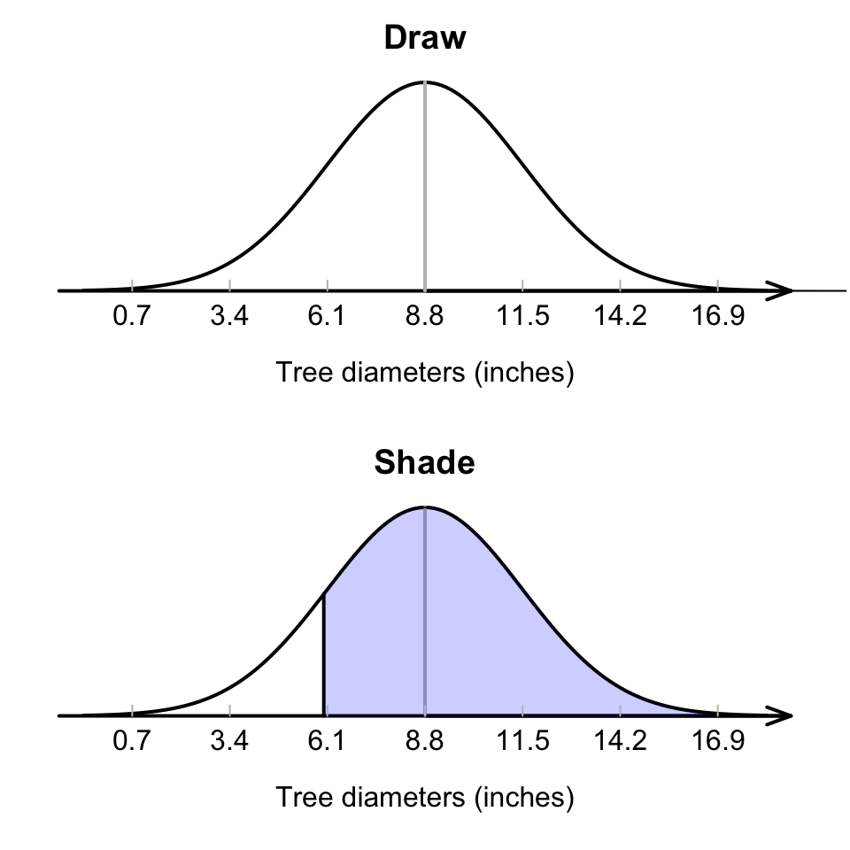
FIGURE 17.7: What proportion of tree diameters are greater than 6 inches?
The normal-distribution tables in the Appendix always provide area to the left of the \(z\)-scores that is looked up. Drawing a picture of the situation is important: it helps visualise how to get the answer from what the table give us.
Remember: The total area under the normal distribution is one.Think 17.1 (Drawing diagrams) Match the diagram in Fig. 17.8 with the meaning for the tree-diameter model (recall: \(\mu=8.8\) inches):
- Tree diameters greater than 11 inches.
- Tree diameters between 6 and 11 inches.
- Tree diameters less than 11 inches.
- Tree diameters between 3 and 6 inches.
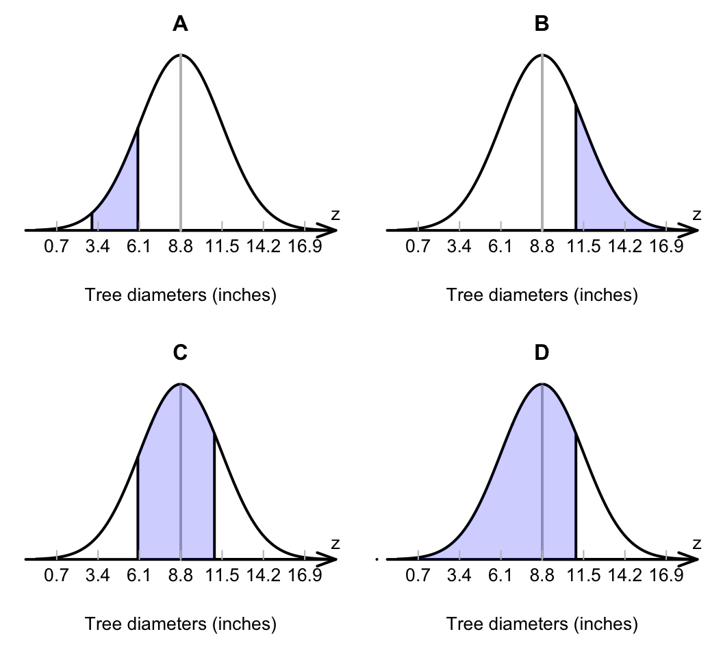
FIGURE 17.8: Match the diagram with the description
First, draw the situation, and shade ‘between 6 and 10 inches’ (Fig. 17.9). Then, compute the \(z\)-scores for both tree diameters:
\[\begin{align*} \text{6 inches: } &z = \displaystyle \frac{6 - 8.8}{2.7} = -1.04;\\[6pt] \text{11 inches: } &z = \displaystyle \frac{11 - 8.8}{2.7} = 0.81. \end{align*}\] Table B can then be used to find the area to the left of \(z = -1.04\), and also the area to the left of \(z = 0.81\). However, neither of these provide the area between \(z = -1.04\) and \(z = 0.81\) (Fig. 17.10).
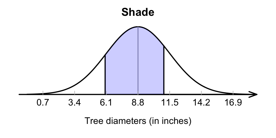
FIGURE 17.9: What proportion of tree diameters are between 6 and 11 inches?
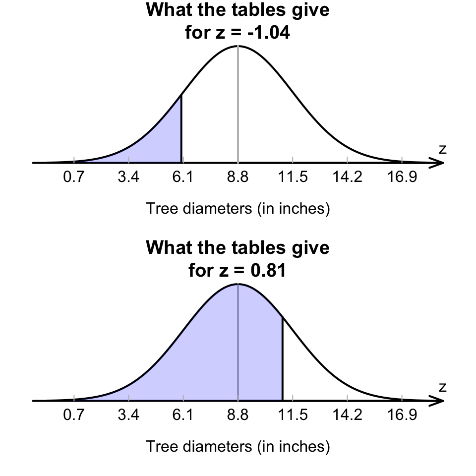
FIGURE 17.10: What proportion of tree diameters are between 6 and 11 inches? The two shaded areas given are what we find by using the tables with \(z=-1.04\) and \(z=0.81\), but neither give us the area we are seeking
Looking carefully at the areas from the tables and the area sought, that area between the two \(z\)-scores is
\[ 0.7910 - 0.1492 = 0.6418; \] see the animation below. The probability that a tree has a diameter between 6 and 11 inches is about 0.6418, or about 64%.
Click on the hotspots in the following image, to see what the areas under the normal curve mean.