23.10 Example: Blood pressure

A US study (Schorling et al. 1997; Willems et al. 1997) examined how CHD risk factors were assessed among parts of the population with diabetes. Subjects reported to the clinic on multiple occasions. Consider this RQ:
What is the mean difference in diastolic blood pressure from the first to the second visit?
Each person has a pair of diastolic blood pressure (DBP) measurements: One each from their first and second visits. The data (shown below) are from the 141 people for whom both measurements are available (some data are missing). The differences could be computed as:
- The first visit DBP minus the second visit DBP: the reduction in DBP; or
- The second visit DBP minus the first visit DBP: the increase in DBP.
Either way is fine, provided the order is used consistently. Here, the observation from the second visit will be used, so that the differences represent the reduction in DBP from the first to second visit.
The parameter is \(\mu_d\), the population mean reduction in DBP.
Since the data set is large, the appropriate graphical summary is a histogram of differences (Fig. 23.4). The numerical summary can summarise both the first and second visit observations, but must summarise the differences. Numerical summaries can be computed using software, then reported in a suitable table (Table 23.3).
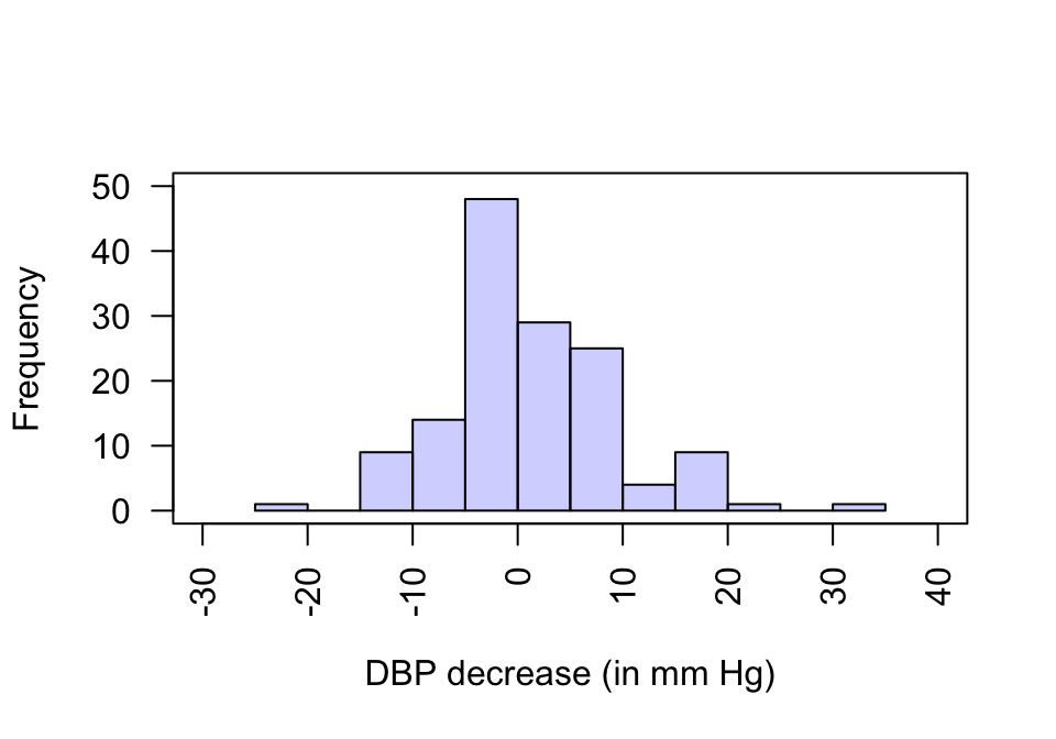
FIGURE 23.4: Histogram of the decrease in DBP between the first and second visits
| Mean | Standard deviation | Standard error | Sample size | |
|---|---|---|---|---|
| DBP: First visit | 94.48 | 11.473 | 0.966 | 141 |
| DBP: Second visit | 92.52 | 11.555 | 0.973 | 141 |
| Decrease in DBP | 1.95 | 8.026 | 0.676 | 141 |
The standard error of the sample mean is
\[ \text{s.e.}(\bar{d})=\frac{s_d}{\sqrt{n}} = \frac{8.02614}{\sqrt{141}} = 0.67592. \] Using an approximate multiplier of 2, the margin of error is:
\[ 2 \times 0.67592 = 1.3518, \] so an approximate 95% CI for the decrease in DBP is
\[ 1.9504\pm 1.3518, \] or from \(0.60\) to \(3.30\) mm Hg, after rounding sensibly. We write:
Based on the sample, an approximate 95% CI for the mean decrease in DBP is from \(0.60\) to \(3.30\) mm Hg.
The exact 95% CI from jamovi (Fig. 23.5) or SPSS (Fig. 23.6), using an exact \(t\)-multiplier rather than an approximate multiplier of 2, is similar since the sample size is large. After rounding, write:
Based on the sample, an exact 95% CI for the decrease in DBP is from \(0.61\) to \(3.29\) mm Hg.
The wording (‘for the decrease in DBP’) implies which reading is the higher reading on average: the first.
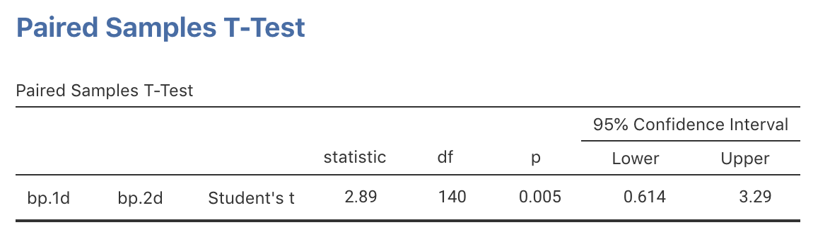
FIGURE 23.5: jamovi output for the blood pressure data, including the exact 95% CI
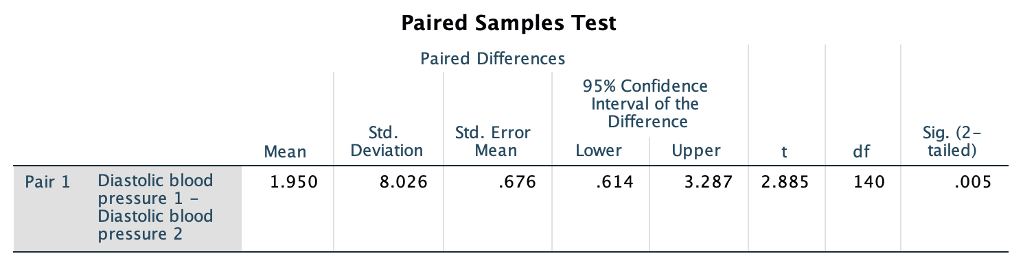
FIGURE 23.6: SPSS output for the blood pressure data, including the exact 95% CI
The CI is statistically valid as the sample size is larger than 25. (The data do not need to follow a normal distribution.)