34.4 Hypothesis testing
34.4.1 Introduction
For the red deer data (Sect. 33.2; Sect. 34.1), the population correlation coefficient between the weight of molars \(y\) and age of the deer \(x\) is unknown and denoted by \(\rho\). The sample correlation coefficient is \(r = -0.584\), but the value of \(r\) varies from sample to sample (there is sampling variation).
The size of the sampling variation is measured with a standard error. However, there is a complication for correlation coefficients17; so we will not produce CIs for the correlation coefficient.
34.4.2 Hypothesis testing details
As usual, questions can be asked about the relationship between the variables, as measured by the unknown population correlation coefficient:
Is the population correlation coefficient zero, or not?
In the context of the red deer data:
In male red deer, is there a correlation between age and the weight of molars?
The RQ is about the population parameter \(\rho\). Clearly, the sample correlation coefficient \(r\) is not zero, and the RQ is asking whether this could be attributed to sampling variation. The null hypotheses is:
- \(H_0\): \(\rho = 0\)
The parameter is \(\rho\), the population correlation between the age and molar weight in the red deer.
This is the usual ‘no relationship’ position, which proposes that the population correlation coefficient is zero. The alternative hypothesis is:
- \(H_1\): \(\rho \ne 0\)
This is a two-tailed test here, based on the RQ.
The approach is to assume that \(\rho=0\) (from \(H_0\)), then describe what values of \(r\) could be expected, under that assumption, just through sampling variation. Then the observed value of \(r\) is compared to the expected values to determine if the valuew of \(r\) supports or contradicts the assumption.
Software is used to test the hypotheses;
the output in
Figs. 34.5 (jamovi)
and 34.6 (SPSS)
contains the relevant \(P\)-value
(twice in the SPSS output!).
The two-tailed \(P\)-value for the test
(labelled Sig. by SPSS) is less than 0.001
(0.000 in SPSS).
That is,
the \(P\)-value is zero to three decimal places,
so there is very strong evidence to support \(H_1\)
(that the correlation in the population is not zero).
We write:
The sample presents very strong evidence (two-tailed \(P < 0.001\)) of a correlation between molar weight and the age of the male red deer (\(r = -0.584\); \(n=78\)) in the population.
Notice the three features of writing conclusions again: An answer to the RQ; evidence to support the conclusion (‘two-tailed \(P < 0.001\)’; no test statistic is given); and some sample summary information (‘\(r = -0.584\); \(n=78\)’).
The evidence suggests that the correlation is not zero (in the population). However, a non-zero correlation doesn’t necessarily mean a strong correlation.
The correlation may be weak in the population (as estimated by the value of \(r\)), but there is evidence that it is not zero in the population.This may be a useful analogy: If a rain forecast says ‘there is a very high chance of rain tomorrow,’ it doesn’t mean there will be a lot of rain, just a high chance of some rain.
34.4.3 Statistical validity conditions
As usual, these results hold under certain conditions to be met. The conditions for which the test is statistically valid are:
- The relationship is approximately linear.
- The variation in the response variable is approximately constant for all values of the explanatory variable.
- The sample size is at least 25.
The sample size of 25 is a rough figure here, and some books give other values.
In addition to the statistical validity condition, the test will be externally valid if the the sample is a simple random sample from the population. The test will also be internally valid if the study was well designed.
Example 34.5 (Statistical validity) For the red deer data, the scatterplot (Fig. 33.2) shows that the relationship is approximately linear, and the variation in molar weights doesn’t seem to be obviously getting larger or smaller for older deer, so correlations are sensible. The sample size is also greater than 25.
The test in Sect. 34.4 will be statistically valid.Example 34.6 (Statistical validity) A study (Schepaschenko et al. 2017; Dunn and Smyth 2018) examined the foliage biomass of small-leaved lime trees. A plot of the foliage biomass against diameter (Fig. 34.7) shows that the relationship is non-linear. In addition, the variation in foliage biomass increases for larger diameters (for values of \(x\) near 10, the values of \(y\) do not vary much at all, but for values of \(x\) near 30, the values of \(y\) vary greatly).
Both of these issues mean that correlations are not appropriate. A hypothesis test similar to that in Sect. 34.4 is inappropriate.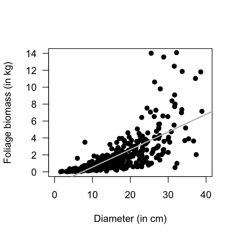
FIGURE 34.7: Foliage biomass plotted against diameter for small-leaved lime trees
References
For those who want to know: the value of \(r\) only varies between \(-1\) and \(1\), so the sampling distribution is not a normal distribution. Instead, a transformation of the correlation coefficient has an approximate normal distribution and standard error. Software automatically does this transforming.↩︎