18.2 Looking at several variables in one plot

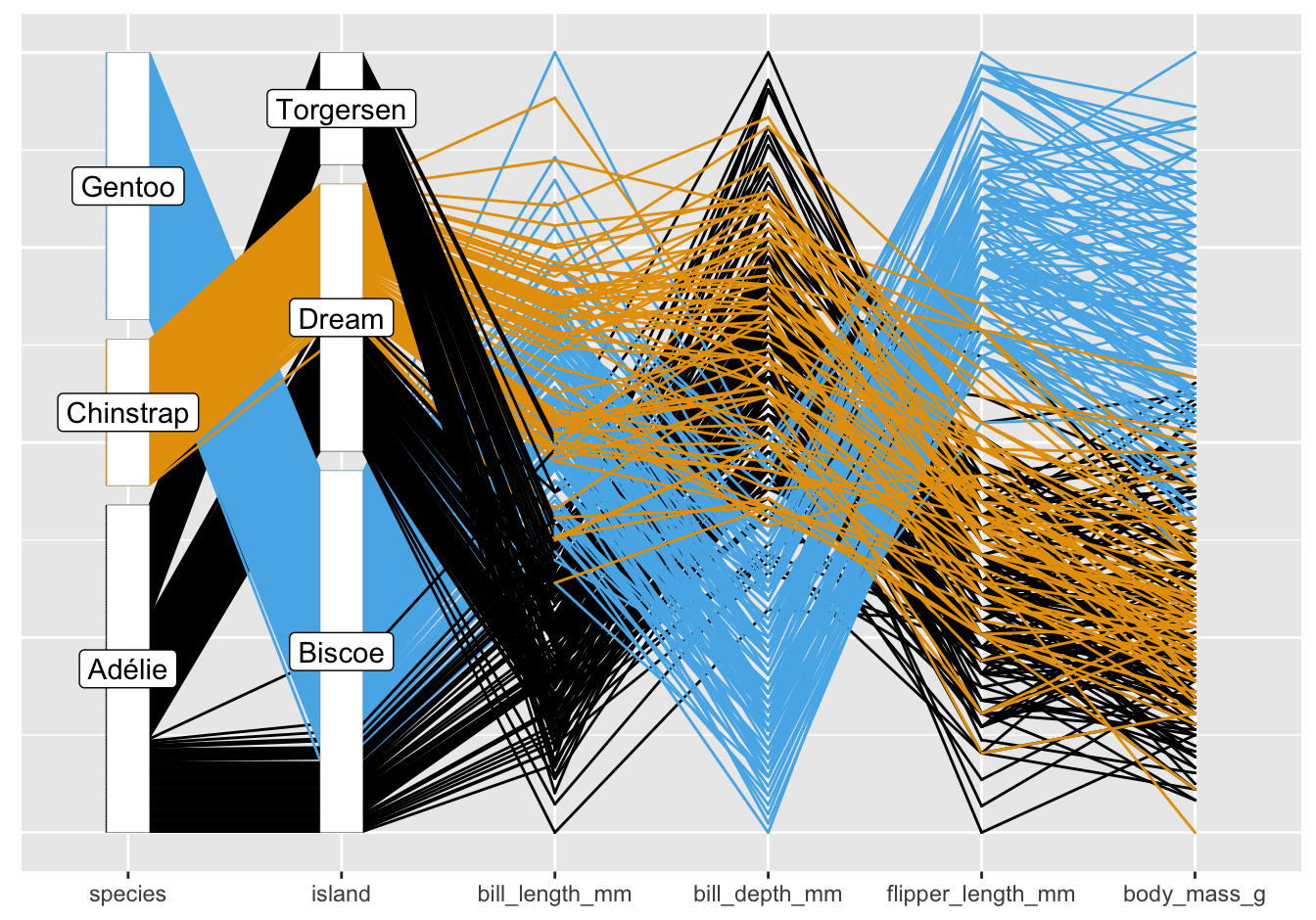
Examining all variables together can be helpful in determining which differentiate between the species. Figure 18.7 is a parallel coordinate plot of the data with the cases coloured by species.

Figure 18.7: Parallel coordinate plot of the Palmer Penguin data

The first two axes show the information already seen in Figures 18.2 and 18.3 that Gentoo penguins are only to be found on Biscoe and Chinstrap penguins only on Dream. Other features can be seen too, such as the different patterns between bill length and bill depth for the species.

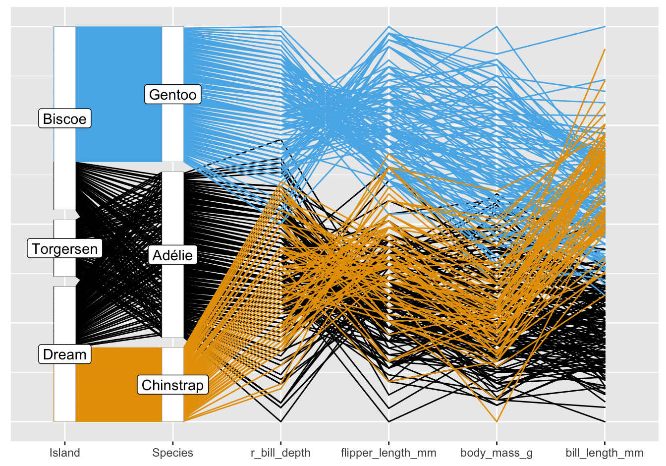
Further features may be separated out better in a parallel coordinate plot by reordering categories and variables. Chinstrap are only on Dream Island, so those categories should be at the top or bottom, and Gentoo are only on Biscoe Island, so they should be at the other end. It also seems better to place island before species. Most measurements have higher values for Gentoo penguins, but bill depth has lower values, so it could be reversed to reduce the numbers of line crossings. Finally, bill length has a different pattern to the other measurement variables and so might be moved to the far right. Figure 18.8 shows the data with the species and islands reordered, with bill depth reversed, and variables reordered.

Figure 18.8: Reordered parallel coordinate plot of the Palmer Penguin data

In this display Chinstrap and Adélie penguins have similar measurement distributions, apart from bill length: Chinstrap penguins have longer bills. Gentoo penguins have higher values on several variables, except for bill depth—remember that this variable has been reversed in Figure 18.8. The fact that all blue (Gentoo) crossings between reversed bill depth and flipper length are above all other crossings between the two variables means that together they separate Gentoo from the other species.

There may be a more effective reordering of the categories and variables. Minimising the total number of line crossings could be a goal or, given the aim of distinguishing between the species, minimising the number of line crossings of different species, but how would a search through the myriad options be carried out? There are 6!=720 orderings of the six variables, 3!=6 orderings of the islands, 3!=6 orderings of the species, and \(2^{4}\)=16 ways of mapping the variables (each one can be plotted as is or inverted). Some of these are equivalent (a reverse ordering of the variables will give the same result as an unreversed ordering), but there does not appear to be an obvious search procedure.

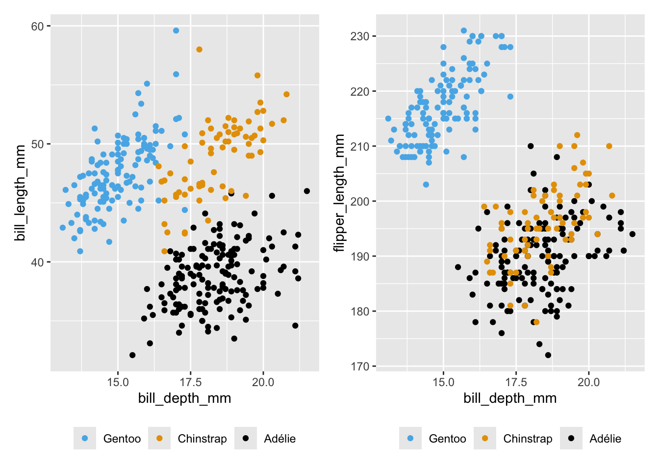
Bivariate associations seen in parallel coordinate plots can be examined more closely with scatterplots. Figure 18.9 confirms how bill length and bill depth combined separate the species (left) and how bill depth and flipper length combined separate Adélie penguins from the other two species (right).

Figure 18.9: Scatterplots of bill depth with bill length and flipper length

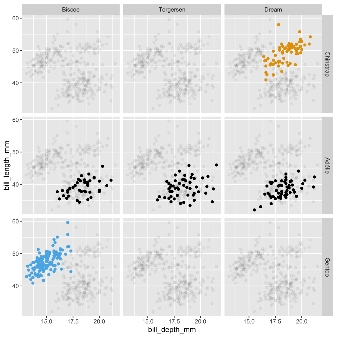
Another way of exploring groups is to use facets. Figure 18.10 shows bill lengths and depths for each combination of species and island. To aid comparisons, the plot for all the penguins has been drawn in the background.

Figure 18.10: Scatterplots of bill lengths and depths of penguins by the three species and three islands

Whichever graphics or tables are drawn to investigate this dataset, it is quickly clear that the Chinstrap penguins are only found on Dream Island and that the Gentoo penguins are only found on Biscoe Island. Fig 18.10 shows that the association between bill length and depth is positive for all species on any island they are found on. It also suggests, if you look at the subplots with no highlighted cases, that the association between bill length and depth for all penguins together is negative. The calculated correlation for the whole dataset is -0.24, while the correlations for the highlighted groups in the individual facets range from 0.25 to 0.65.