8.4 Ratings change over time

FIDE’s website used to offer datasets going back to January 2001. Currently it offers almost 8 years of monthly ratings datasets and also ratings charts for individual players going back 20 years. The ratings in December 2020 were unusual because tournaments had not taken place due to the Covid pandemic. The December 2015 ratings were chosen for comparison.

The January 2001 dataset only includes players with a rating of over 2000 and has just 36979 players, slightly over a tenth of the number for December 2020. The December 2015 list has no rating restriction, but only 227960 players, so there were about 59% more at the end of 2020, five years later. The proportion of players flagged as inactive has also gone up from 42% to 47% and that explains part of the difference in overall numbers.

Figure 8.14 compares the densities of the rating distributions of active players in December 2015 and December 2020. The difference in the distributions is striking and it might be that there was a higher proportion of young active players in 2020.

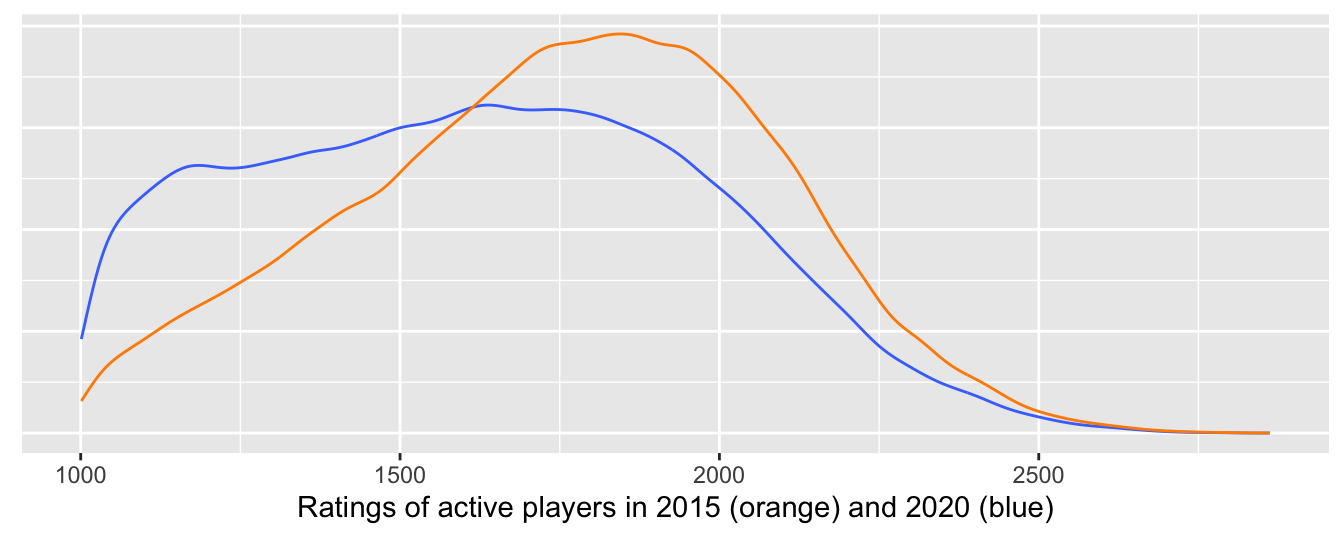
Figure 8.14: Density estimates of distributions of ratings in December 2015 and December 2020

Figure 8.15 compares density estimates of players’ ages and confirms that there was a higher proportion of younger active players in 2020.

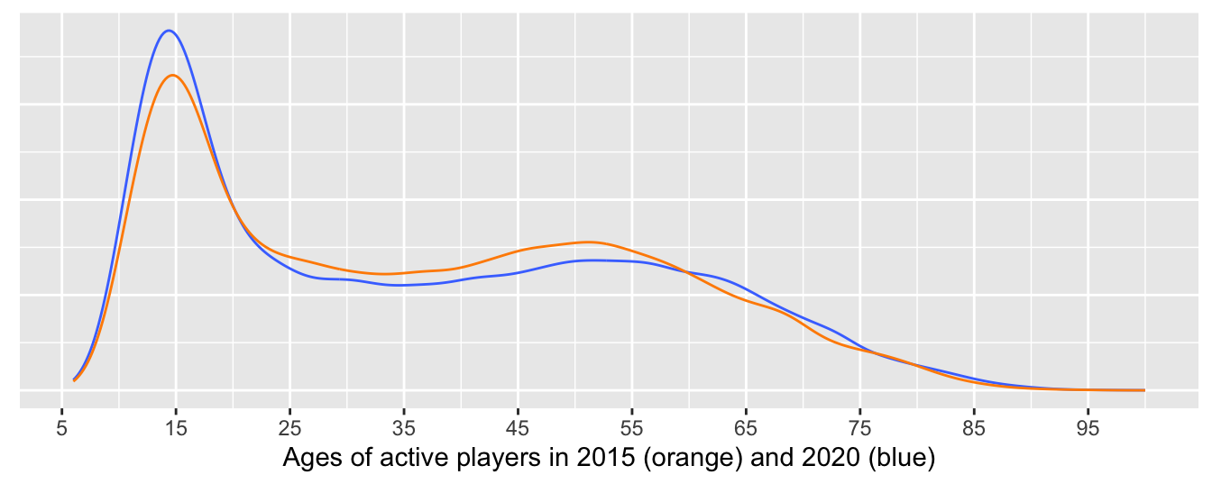
Figure 8.15: Density estimates of active players’ ages in 2015 and 2020

Ratings can be plotted against age in a scatterplot to study how they depend on age. Usually statisticians want more data than they have, so that they can study their data in greater depth. With the chess ratings there is almost too much data! Figure 8.16 illustrates the problem for the December 2015 data. 132489 points have been plotted and there are many overlapping points. An alpha value of 0.05 means that only locations where there are 20 or more points are completely black. This alpha value is too high where there is a lot of data (the very young) and too low where there is little data (the top rated players). Nevertheless we can see that there are no very young high-rated players and that there are relatively few low-rated players aged over 20 or so. There is a decline in the numbers of the very top-rated players with increasing age.

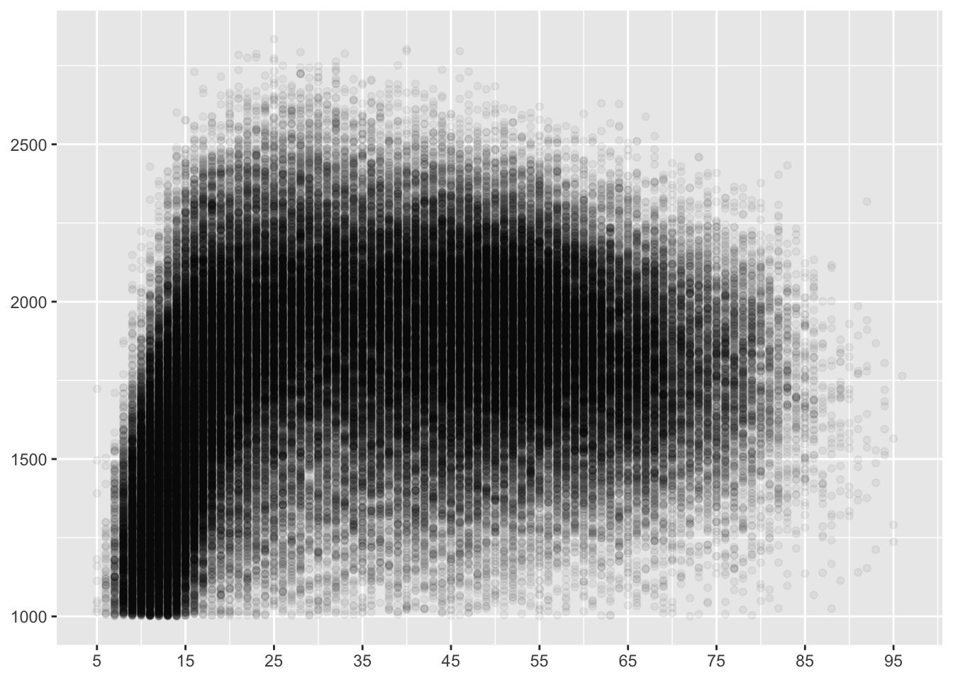
Figure 8.16: Rating by age for active players in 2015 (an alpha value of 0.05 has been used)

The bulk of the players form a shape like a short-necked bird with a long head, perhaps a brent goose. The discreteness of the age data is noticeable due to the striping effect of the gaps. It would not arise with exact ages. The points could be made bigger, but then there would just be one big black blob.

One approach would be a form of two-dimensional density estimation or hexagonal binning (Carr et al. (1987)), possibly including jittering of the age values. Since the dataset is a December one it can be safely assumed that almost all players are at least the calculated age, so that if jittering is carried out it should be by adding a jitter term from [0,1).

A way to both show the densest parts of the data and pick out the top-rated players would be to colour the points for those top players and use different alpha values for the two groups. Figure 8.17 uses an alpha of 0.01 for most of the data and an alpha of 1 for the 44 players coloured red with ratings over 2700.

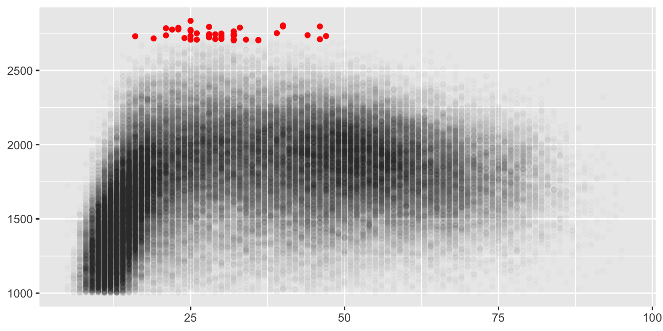
Figure 8.17: Rating by age for active players in 2015 (players with ratings over 2700 are coloured red and an alpha value of 0.01 has been used for the others)

Simplest would be to take a random sample and this has been done in Figure 8.18 using a 10% sample and alpha=0.1. The advantage of sampling from a large dataset is that even a much smaller sample than this 10% one would give an excellent estimate of the overall structure and it is not necessary to draw so many points for that purpose. To be on the safe side a second or even a third sample could be taken to check any results. The disadvantage is that anything rare, such as outliers or unusual cases, may not be included in the samples.

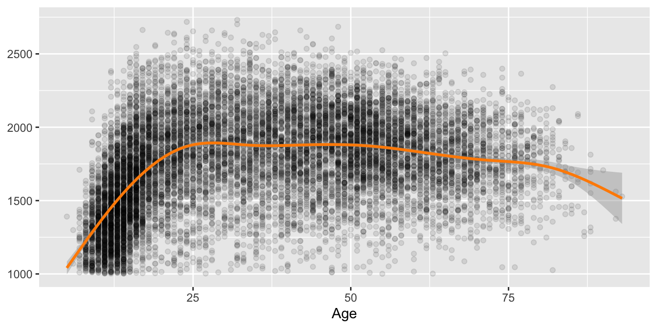
Figure 8.18: Rating by age for a 10% sample of active players in 2015 with a nonlinear smooth and confidence band

Another alternative, using the enforced discreteness of the age variable, would be to draw boxplots for each age (Figure 8.19). The 38 players over 90 have been excluded as have the 2889 players whose year of birth is not known. The medians of the boxplots show the same pattern as the smooth in Figure 8.18, as do the upper and lower hinges of the boxplots, and the display gives a clear picture of where the middle 50% of the data lie at each age. The upper outliers are players who are exceptional for their age and the lower outliers are players who still compete although they are weak. The first lower outlier appears at age 23, perhaps an indication that many weaker players have given up by then.

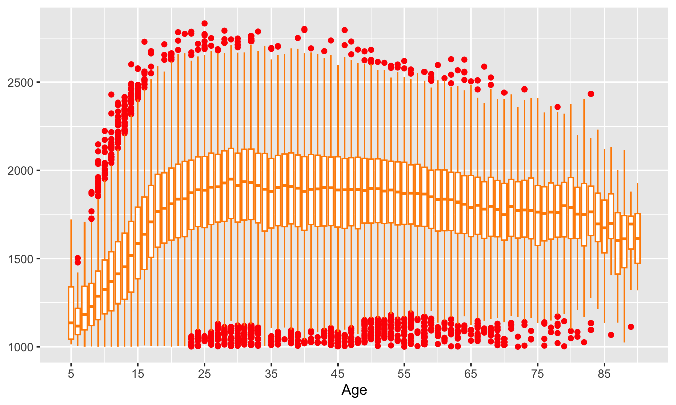
Figure 8.19: Boxplots of ratings by age for active players in 2015

The disadvantage of using boxplots is that they cannot show multimodality, if it exists. To check for multimodality, consider ridge plots, as in Figure 8.20. Most of the ridges look close to unimodal, symmetric distributions. Ridges have only been drawn here for ages at every 5 years for the main part of the dataset from ages 15 to 65. While ridges are good for the central bulk of distributions they are not so good at the extremes where they may imply higher or lower values than are reasonable. As no players can have ratings less than 1000, an option has been chosen to set a boundary there. Similarly, the upper tails of the distributions have been bounded. Using ridgeplots and boxplots in combination is a promising solution.

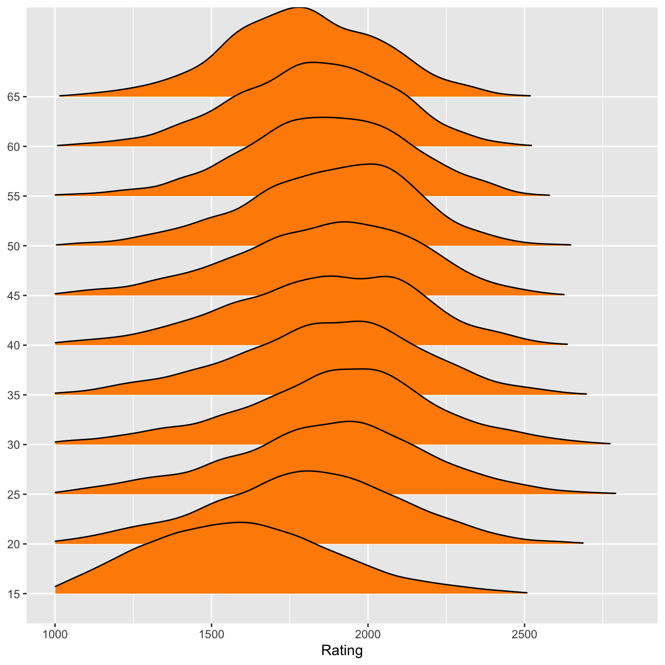
Figure 8.20: Ridgeplots of ratings for active players in 2015 for ages from 15 to 65 in 5 year jumps

Returning to comparing the rating datasets in December 2015 and 2020, Figure 8.21 shows two scatterplots of rating by age, one for the active players in the December 2015 dataset and one for the active players in the December 2020 dataset. Smooths have been drawn to show how rating varies with age.

Figure 8.21: Rating by age for active players in 2015 and 2020

The scatterplots look fairly similar in form. A direct comparison of the smooths is shown in Figure 8.22.

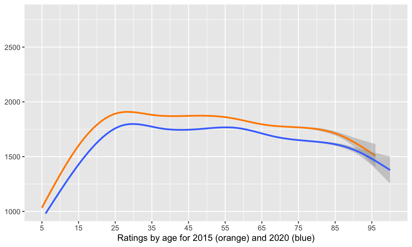
Figure 8.22: Smooths for ratings by age for active players in 2015 and 2020

Smoothed ratings by age for active players were uniformly lower in 2020 than in 2015. This is likely because there were many more active players in 2020 than in 2015. It is curious that the smooth for 2020 starts at a higher age than the one for 2015. Exploring the data showed that there were fewer very young rated players in 2020. The data reveal that there were 0 five-year-olds in the 2020 dataset and only 12 six-year-olds (in 2015 the corresponding numbers were 10 and 52). This was probably due to the pandemic leading to few tournaments being played, so that the very youngest players could not get started.

8.4.1 Individual players

The changes between December 2015 and December 2020 could be explored further by looking at the three populations of players involved: those who appear in both lists, those who were present in 2015 but not in 2020, and the new ones.

Merging the two data files by player ID number reveals that 226450 players appear in both lists, 1510 players are on the 2015 list, but not on the 2020 list, and 136052 players are only on the 2020 list. It seems to be much harder to leave the ratings list than to join it!

Rather than studying population changes between two particular time points, it would be more informative to create a longitudinal dataset by combining all the rating datasets and studying players’ career paths over the months and years.