26.2 Are there geographic patterns?
There are strong geographic patterns in party support across the constituencies. Figure 26.7 shows support for the Greens in choropleth maps.
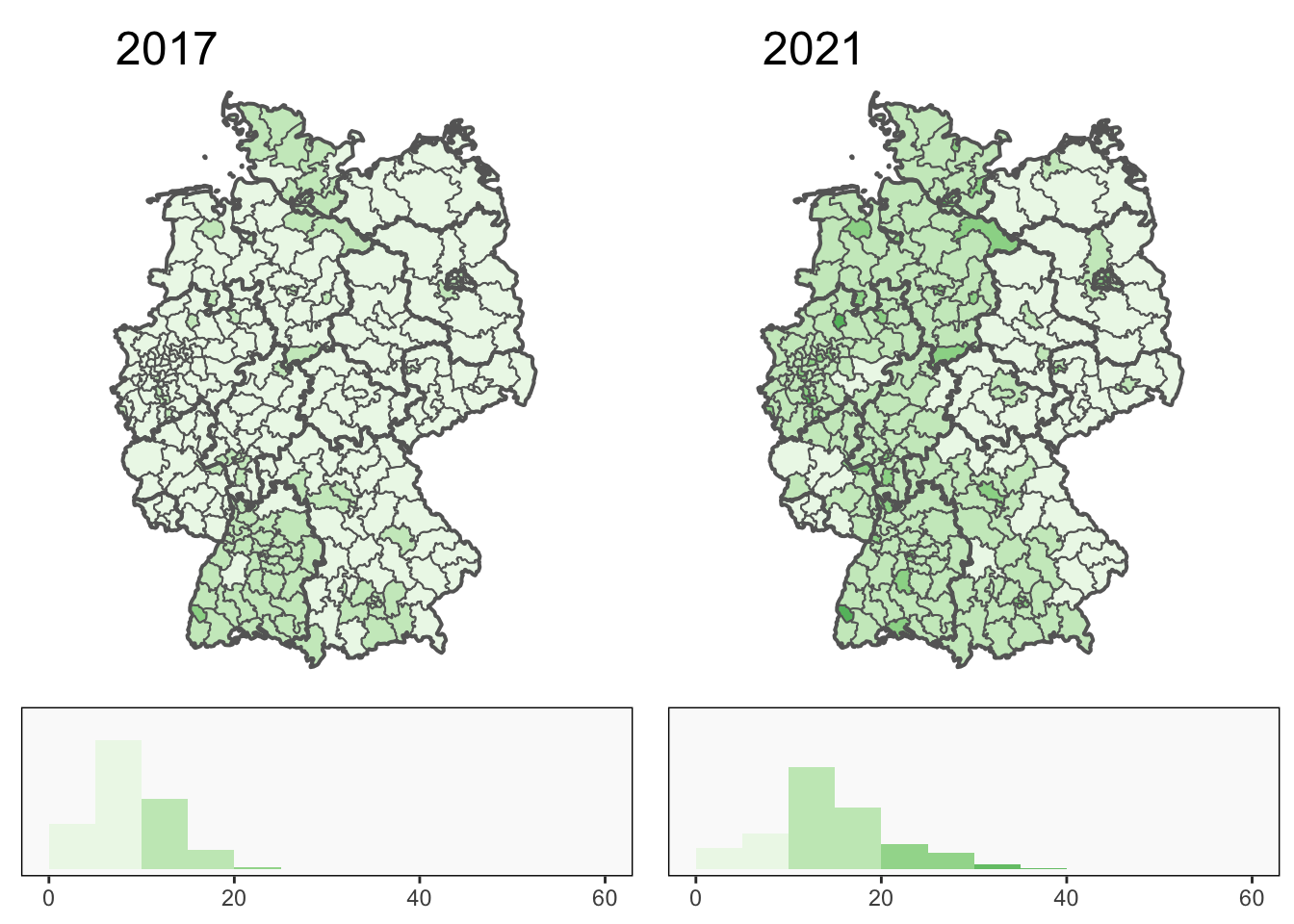
Figure 26.7: Percentage Green support across the constituencies in 2017 (left) and 2021 (right). Bundesland borders are drawn in thick black. The colour scale goes from 0 to 60 in intervals of 10 (histograms below).
The Greens did much better in 2021, predominantly in the West of Germany. They also did better in more densely populated areas, as Figure 26.8 shows using the logarithm of population density as a measure.
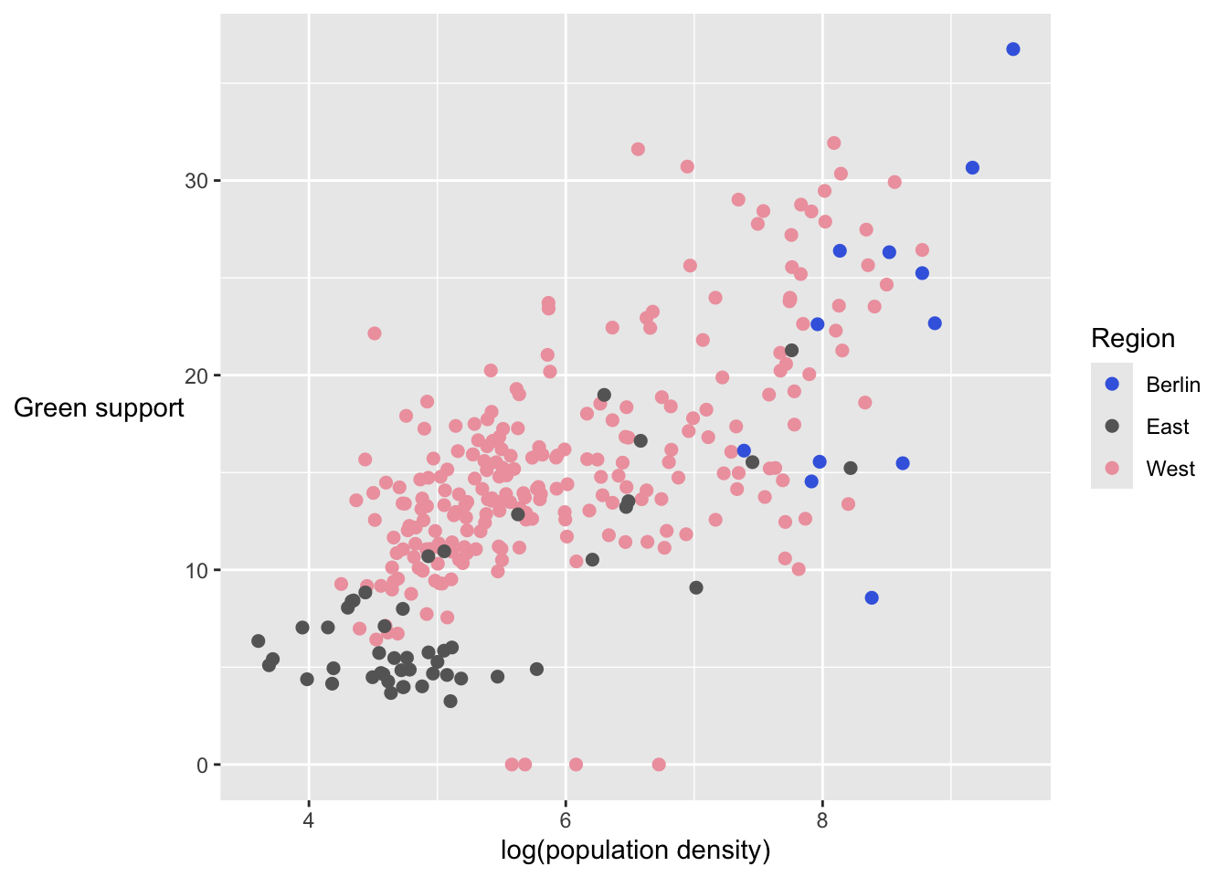
Figure 26.8: Green support plotted against log of population density
Aside from the four constituencies of Saarland where the Greens got no party votes, as already mentioned, there is a roughly linear relationship in the plot. The Greens did worst in the rural East and best in big cities including parts of Berlin. There is a little overplotting in Figure 26.8, so the points representing West were drawn first and the smaller East and Berlin groups on top.
Associations with other variables can be explored using a parallel coordinate plot (Figure 26.9). The Greens did well where there were more younger people and where there were more qualified to go to university.
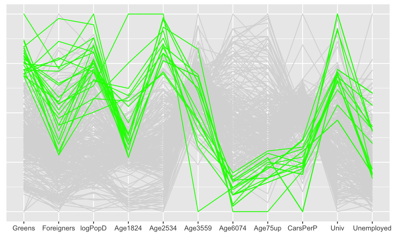
Figure 26.9: A parallel coordinate plot of Green support and some structural variables (constituencies with over 25% Green party votes are coloured green)
The AfD lost ground between the two elections and were weaker in the West.
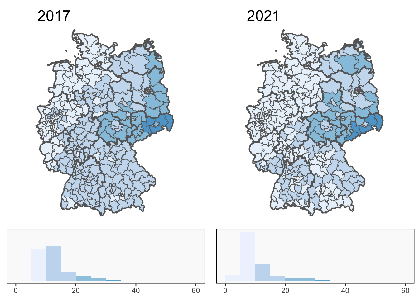
Figure 26.10: Percentage AfD support across the constituencies in 2017 (left) and 2021 (right). Bundesland borders are drawn in thick black. The colour scale goes from 0 to 60 in intervals of 10, as shown in the histograms below.
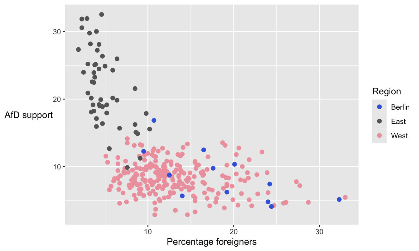
Figure 26.11: AfD support plotted against percentage of foreigners
Figure 26.12 is a parallel coordinate plot of AfD support and the same structural variables as in Figure 26.9. The AfD were strong where there were more older people and low levels of foreigners (people without German nationality). They did not do well in cities, where the population density is higher.
The scatterplot, Figure 26.11, shows more detail of how the AfD vote related to the percentage of foreigners in the constituencies. AfD support is highest where there are few foreigners and relatively constant for any percentage of foreigners a little over 10%. They are generally weaker in the Berlin constituencies than in the rest of the Eastern part of Germany, probably because West Berlin is still different to East Berlin, even over thirty years after reunification. The association may be due to foreigners not voting for the AfD or more due to the party being stronger in the East where there are lower percentages of foreigners.
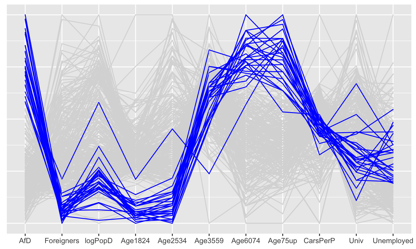
Figure 26.12: A parallel coordinate plot of AfD support and some structural variables (constituencies with over 20% AfD party votes are coloured blue)
The CDU/CSU have traditionally always been strong in Bavaria, the CSU’s part of Germany.
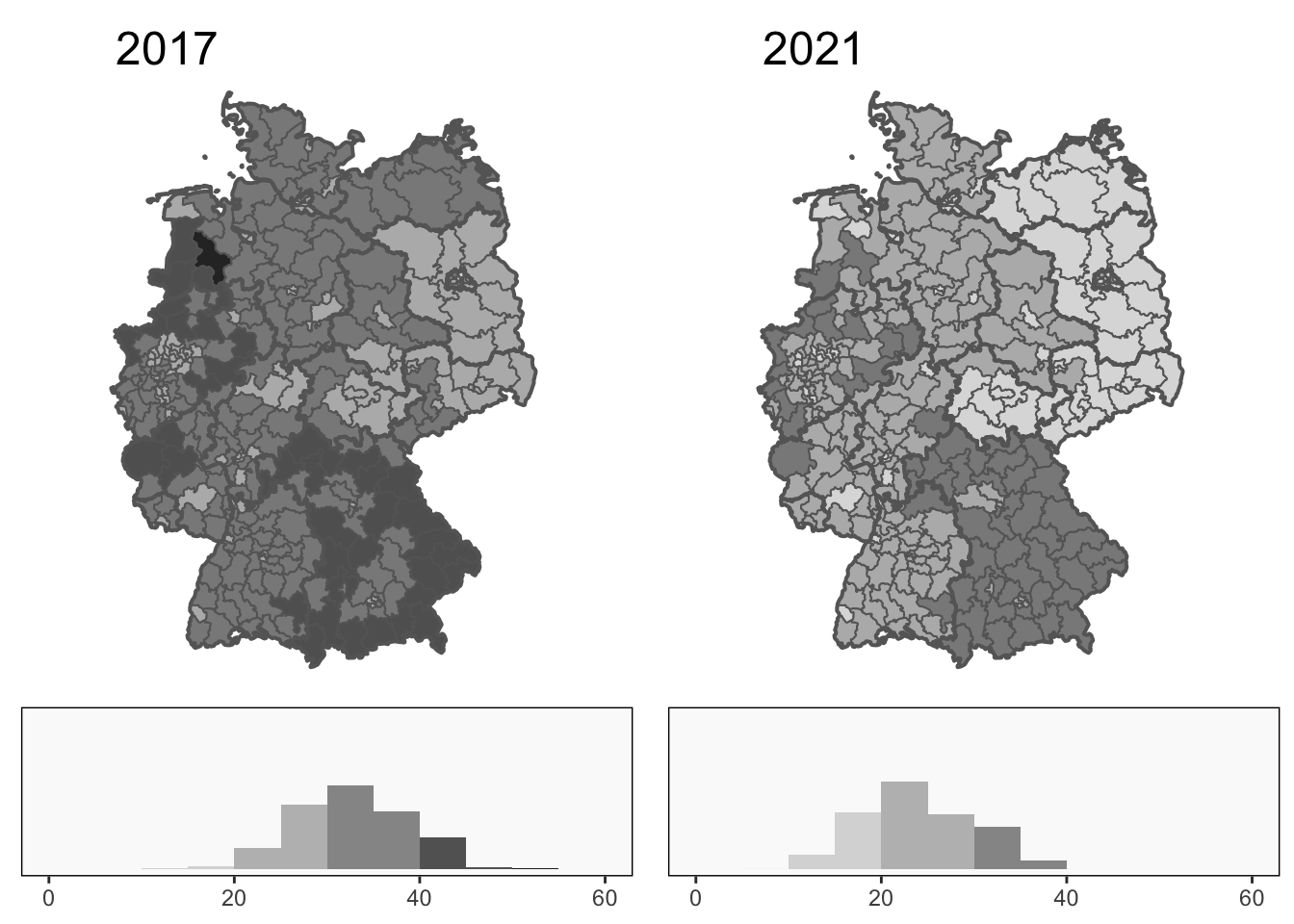
Figure 26.13: Percentage CDU and CSU support across the constituencies in 2017 (left) and 2021 (right). The colour scale goes from 0 to 60 in intervals of 10. Bundesland borders are drawn in thick black.
It is always possible with a large number of factors to find correlations that may or may not imply some causation. For the CDU/CSU one is car ownership, as Figure 26.14 illustrates.
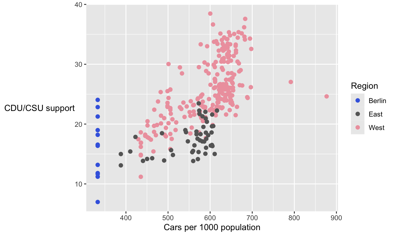
Figure 26.14: CDU and CSU support plotted against numbers of cars per thousand population.
As car density increases, so does support for the CDU and CSU. Car density tends to be lower in the East. The points to the far left are the 12 Berlin constituencies. For major cities car registration statistics are only available for the whole city and so all constituencies have the same (in this case, low) value. Cars are not so useful in large cities. The most outlying value to the right is Wolfsburg, Volkswagen’s main base, and the other one is Main-Taunus, between Opel’s base at Rüsselsheim and Frankfurt.
Drawing a parallel coordinate plot, as for the other two parties, shows that the CDU/CSU additionally did well in areas of lower population density where there were more middle-aged people and fewer unemployed.
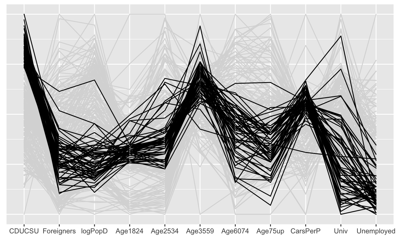
Figure 26.15: A parallel coordinate plot of CDU/CSU support and some structural variables (constituencies with over 30% party votes are coloured black)