31.1 What gets ordered, sorted, arranged?

31.1.1 Cases

Datasets can be sorted and ordered in many ways. The cases in the astronauts dataset on space travel (rfordatascience (2020a)) could be sorted into groups by nationality or sex. They could be ordered by year of mission or by year of birth. They could be sorted and ordered by combinations of these variables, for instance, by year of birth within nationality. Grouping and ordering datasets often reveals structures that default orders—whether lexicographic, temporal or random—may not. Ordering and sorting cases can be useful for checking extreme or special cases quickly. If some text has crept into a numeric variable, sorting can often identify which values are in error.

For sortings or orderings of the astronauts dataset there can be ties, cases that have the same values for the sorting variables, for example people born in the same year of the same nationality. These cases may be ordered randomly amongst themselves or in their original order (whatever that was) or in some other way. Ties would be much less likely if exact dates of birth and exact launch dates of missions were used, although even then pairs like the identical Kelly twins, two Americans, might cause difficulties. To ensure that a return to a particular ordering is always possible, it is essential to have a variable with a unique value for every case, possibly an ID variable constructed for just this reason. Being able to return to the initial order of a dataset is useful if something goes wrong (and something will).

The ordering of cases can affect printing if cases or lines overlap, as the dataset is printed in order. The lines for the three football teams in Figure 16.6 were drawn in alphabetic order, first Bournemouth, then Portsmouth, then Southampton, as can be seen by looking at where the lines cross. (The lines for the other teams in the leagues, drawn in light grey in the background, were drawn in a background layer first.) Figure 11.9 compares calculated values of diamond depth with the values given in the dataset. The data were ordered by the size of the absolute difference, so that the bigger differences, coloured red, were plotted last and hence on top.

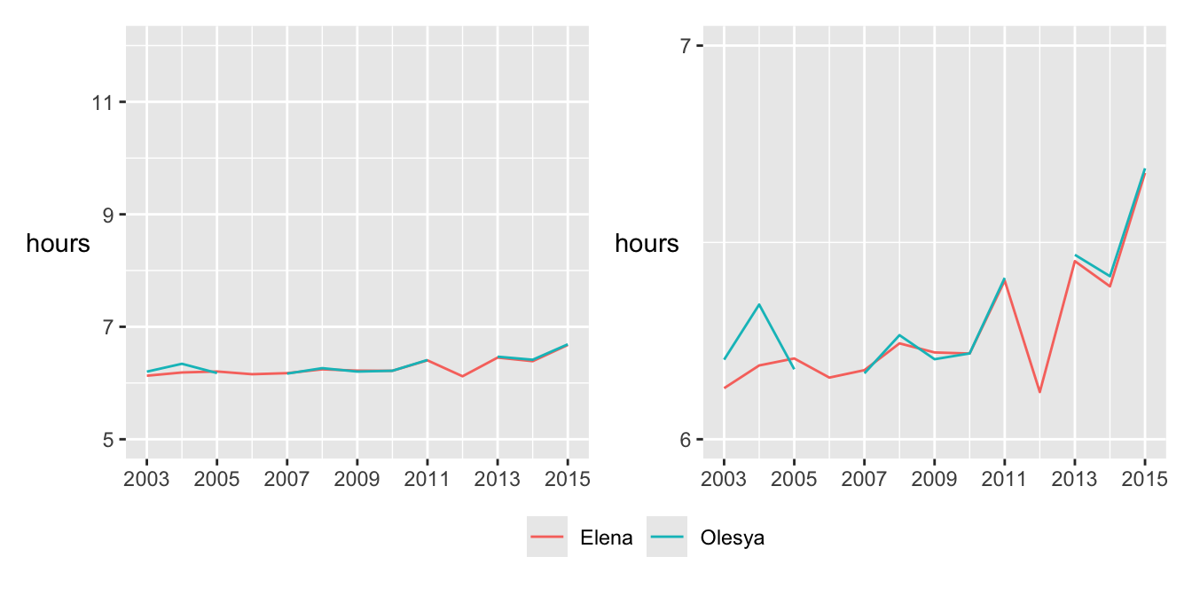
Chapter 21 on the Comrades Marathon includes two plots of the performances of the Nurgalieva twins over the years, Figure 21.13, redrawn here as Figure 31.1. Elena ran every year from 2003 to 2015, while Olesya did not run in 2006 and 2012. In the plots, the line for Olesya is drawn on top. This works if it is remembered that Elena ran every year. If the line for Elena had been drawn on top, that would not have worked, even for the zoomed plot on the right.

Figure 31.1: Performances of the Nurgalieva identical twins in the Comrades Marathon races (same data, different vertical scales)

31.1.2 Levels of categorical variables

Variables such as nationality and occupation each have two or more categories. If you draw up a summary table of counts or draw barcharts of them, the categories are likely to be ordered alphabetically by default. This has its advantages (it is easy to find a category in the table) and its disadvantages (categories with names early in the alphabet get more attention, categories you would like to compare may be far apart). Wainer calls this the “Alabama first” issue, as Alabama comes first alphabetically amongst the US States (Wainer (1997)). Categories may be ordered by counts, by weights, by proportions, by summary statistics on other variables. Comparisons for whatever statistic you order by become easier. Bars far apart must be different and you can tell which bars that are close together have higher or lower values by the order. More complex sortings, say countries within continents, are possible too.

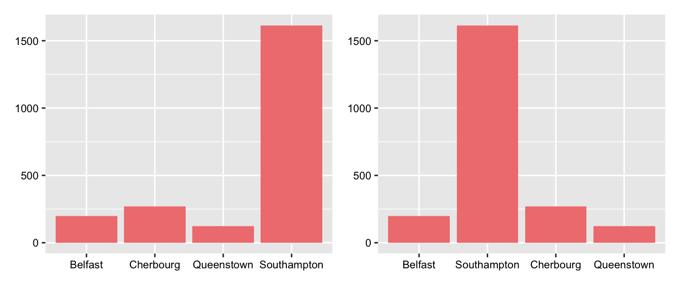
One example is the barchart of the numbers of passengers and crew who boarded the Titanic at the four different ports. Figure 31.2 shows a plot with the default alphabetic ordering on the left and the plot used in §25.1 on the right, using the order the ship called at the ports. The great majority, including many crew, joined in Southampton.

Figure 31.2: Barcharts using the default alphabetic ordering and the order in which the Titanic visited the ports

In the Gapminder analysis, §2.3, there are two barcharts of the four regions, one for the number of countries in each region (Figure 2.7) and one for the total population (Figure 2.8), both ordered by bar heights. The two are shown again here in Figure 31.3. The first shows that Africa and Asia have more countries than Europe or the Americas, while the second shows that Asia has more of the world’s population than the other three regions put together.

Figure 31.3: Numbers of countries and total populations in the four Gapminder regions

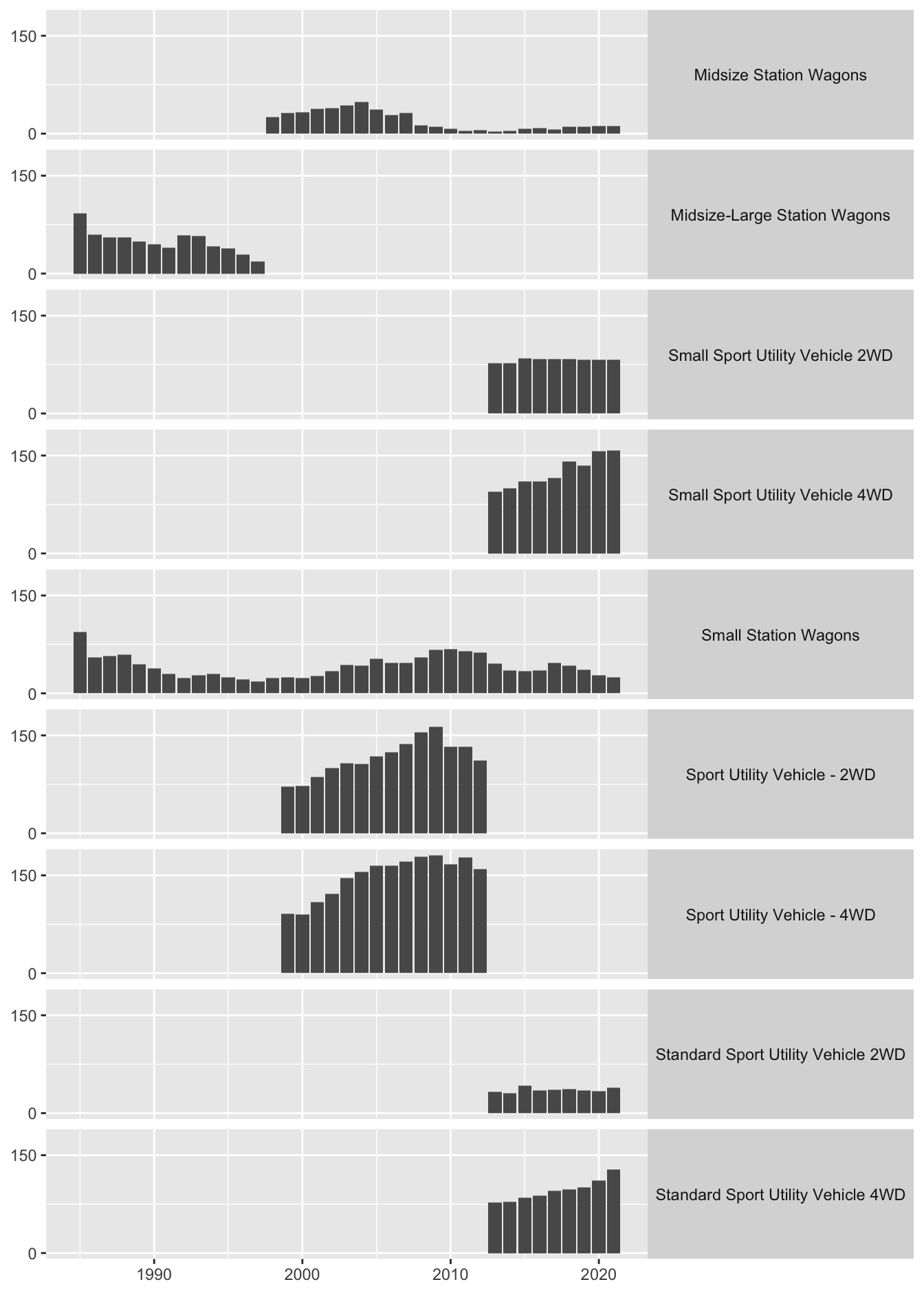
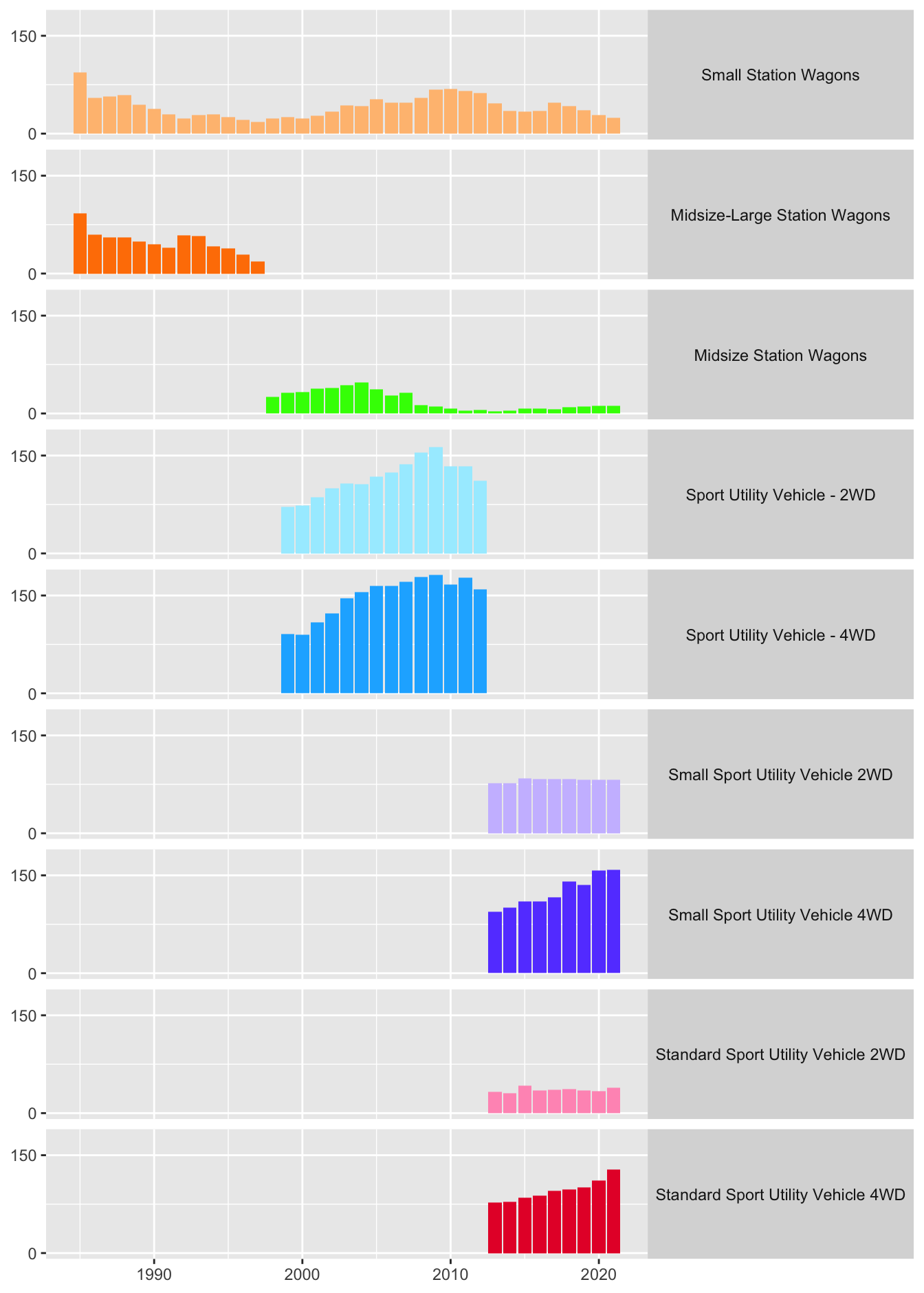
A common reason for reordering categories is to produce a recognisable and memorable pattern, for instance steadily increasing or decreasing. Figure 17.7 shows sales of station wagons and SUVs by year. The original plot is on the right of Figure 31.4 and a plot using a default lexicographic ordering of the vehicle types is on the left.

Figure 31.4: Annual sales of station wagons and SUVs in default ordering (left) and revised ordering (right)

The ordering chosen put the station wagons first and then the SUVs. Within the station wagon group, the models were ordered by increasing size and earliest available production year. Within the SUV group, they were ordered by type using earliest available production year and within that by 2WD and 4WD (two-wheel and four-wheel drive). Multivariate ordering offers many different possibilities, especially when variables are not nested within one another.

31.1.3 Variables

Datasets come with a particular order of variables. There might be an ID variable, some demographic or structural variables, and then some measurements. All of these might be in a rational order, they might not. Datasets with large numbers of variables are easier to handle if the variables are grouped and ordered. The vehicles dataset made available by the US Department of Energy includes 83 pieces of information on 43516 vehicles. The first 65 variables are labelled alphabetically, so that three defining variables, make, model, and year, appear rather late and not together.