11.2 Checking for outliers and unusual values

In all there are \(20\) diamonds with zero values for length, width or depth. All have zero depth, \(8\) have zero length, and of those \(8\), there are \(6\) with zero width. There are no other diamonds with zero width. These \(20\) cases must be errors and might be identified as outliers. Interestingly, outlier detection methods tend not to find them when the whole dataset is used to look for them, probably because they are not far enough away from the rest of the data in multivariate space. After removing the \(20\) zero cases there are still three extreme outliers, two cases with extremely high values of width and one with an extremely high value of depth.

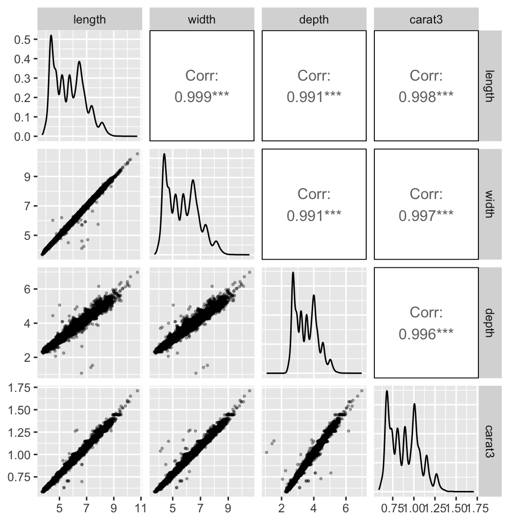
After removing the outliers, a scatterplot matrix of carats and the three dimensions, length, width, and depth identifies other possible outliers. The scatterplots with carat are curved, as it is really a volume measurement, so the cube root of carat was used to get linear plots.

Figure 11.6: A scatterplot matrix of length, width, depth, and carats to the power one third for the dataset after removing the zero cases and three extreme high outliers

The correlations are all very high, despite the apparent variability. The reason is the size of the dataset. Most of the data are linearly related and hidden by overplotting. Several two-dimensional outliers are visible. The three lowest values of depth have middling values of length and width, so the problem is the depth measurement. There are a few other cases that seem too far away from the main body of the data. If a point is a two-dimensional outlier and not an outlier on either of the variables separately, then it could be an error on one or both of the variables or an unusual case. Outliers on individual dimensions are a problem for graphics because they distort the axes and shrink the space available for the main part of the data. This affects one-dimensional plots like histograms, but also higher dimensional displays like scatterplots and parallel coordinate plots.

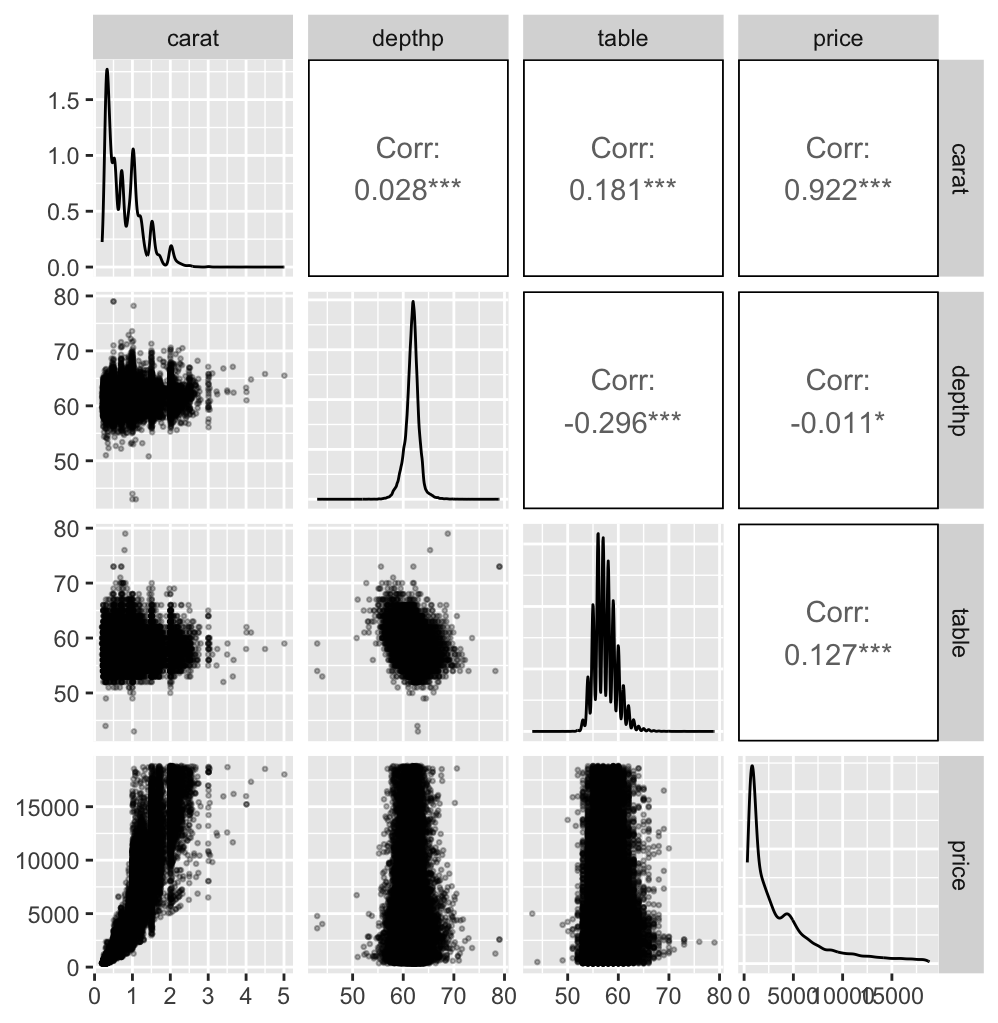
Figure 11.7 shows a scatterplot matrix of carat with the other three continuous variables. An extreme outlier on the variable table has been excluded for the reason just mentioned. A few more cases appear to be outliers. The density estimate for table looks odd. Checking the frequencies of observed values in Figure 11.8 shows that most are integers.

Figure 11.7: A scatterplot matrix of carat, percentage depth, table, and price for the dataset after removing the zero cases and four extreme outliers

Figure 11.8: A vertically jittered dotplot of diamond table, excluding 12 outlying values, showing heaping at integer values

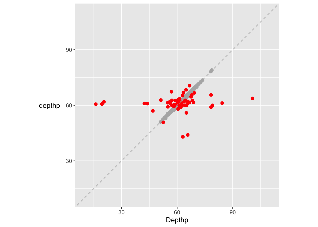
Figure 11.7 shows a few extreme values of percentage depth. According to the R help file for the dataset, percentage depth is calculated from the variables, length, width, and depth. Carrying out the calculation and plotting the reported percentage depth (depthp) against the newly calculated one (Depthp) gives Figure 11.9.

Figure 11.9: A scatterplot of reported percentage depth (depthp) and percentage depth calculated from the data (after removing the zero cases and three extreme outliers). Cases where the difference is bigger than 1 have been coloured red and drawn last.

There are 69 cases where the reported depth percentage and the calculated depth percentage differ by more than 1 and more detailed investigation of the four variables involved would be necessary to determine which cases to keep and/or correct.