18.1 Getting an overview of the penguin data

A good example of the LTER research can be found in Gorman et al. (2014). Some of the data have been made available in the palmerpenguins R package, primarily size measurements and isotopic signature information for three species of penguin: Adélie, Chinstrap, and Gentoo. Colour information is not included, but Gentoo penguins have a distinctive orange bill and white marking above the eyes, while Chinstrap penguins have a narrow black chinstrap. Attractive drawings of the three species are shown on the palmerpenguins package webpage.

The Palmer Archipelago lies to the West of the Antarctic Peninsula, where warming linked to climate change has occurred very fast. According to Fountain (2022) this is bad for Adélie penguins that do better to the East in the Weddell Sea where it is still cold. Gentoo penguins are not so affected.

Figure 18.1 shows four plots of the dataset. There are barcharts for the three species and the three islands, a histogram of penguin body mass, and a scatterplot of flipper length against body mass.

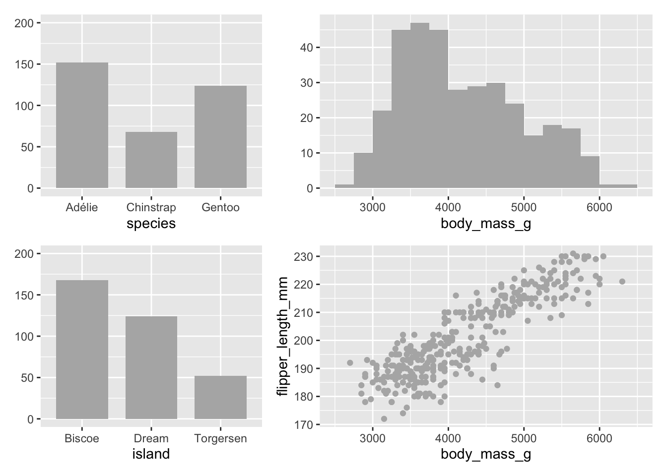
Figure 18.1: Four plots of the Palmer penguin dataset

There are fewer Chinstrap penguins and fewer penguins from Torgersen Island. The distribution of body mass may have that skewed shape because it is a mixture of the body mass distributions of three separate species. Flipper length and body mass are highly positively correlated.

Different subsets can be selected and highlighted to look for patterns. Figures 18.2 and 18.3 show examples of selecting a species or an island across these plots. Gentoo penguins were only sampled on Biscoe Island, and they are generally heavier with longer flippers than the other two species. Dream Island has all the Chinstrap penguins and some Adélie penguins. The penguins on Dream Island have smaller body mass and flipper length.

The penguins in this dataset were nesting pairs that had at least one egg. The sampling procedure is described in Gorman et al. (2014). Detailed information on estimated total penguin numbers at Antarctic sites over the years is available on the MAPPPD website described in Humphries et al. (2017).

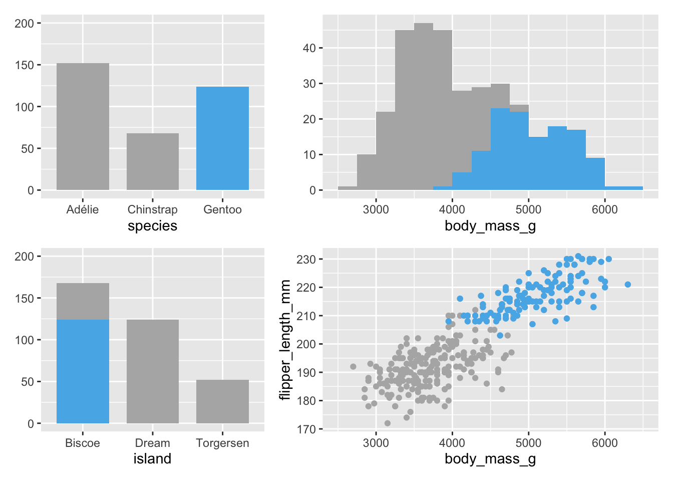
Figure 18.2: Gentoo penguins highlighted in all plots

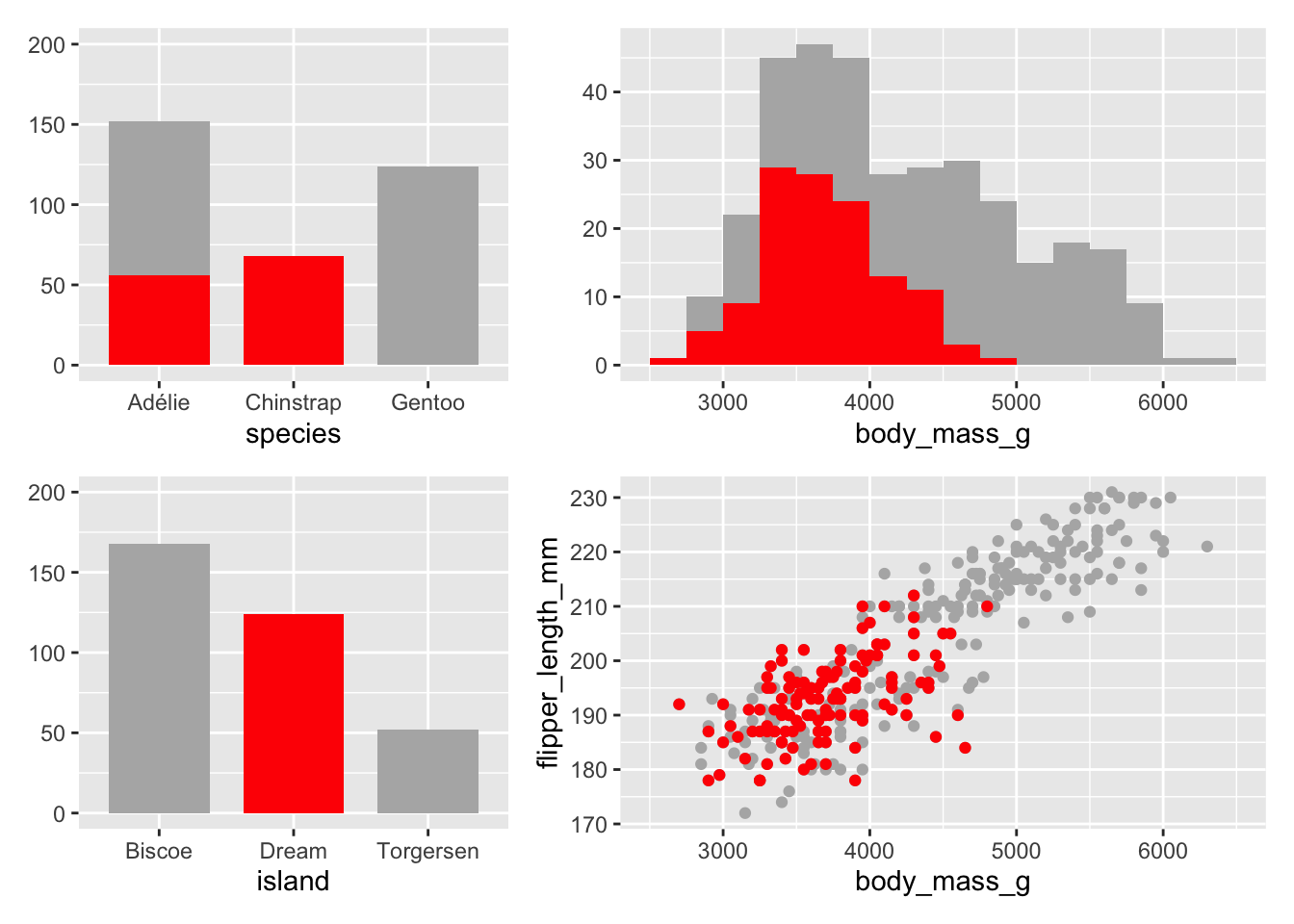
Figure 18.3: Dream Island penguins highlighted in all plots

Groups of cases defined in other ways could also be highlighted. Figure 18.4 highlights the penguins weighing no more than 3 kg. As was already known from Figure 18.2, the penguins are either Adélie or Chinstrap. Interestingly, there are examples of the lightest penguins on all three islands.

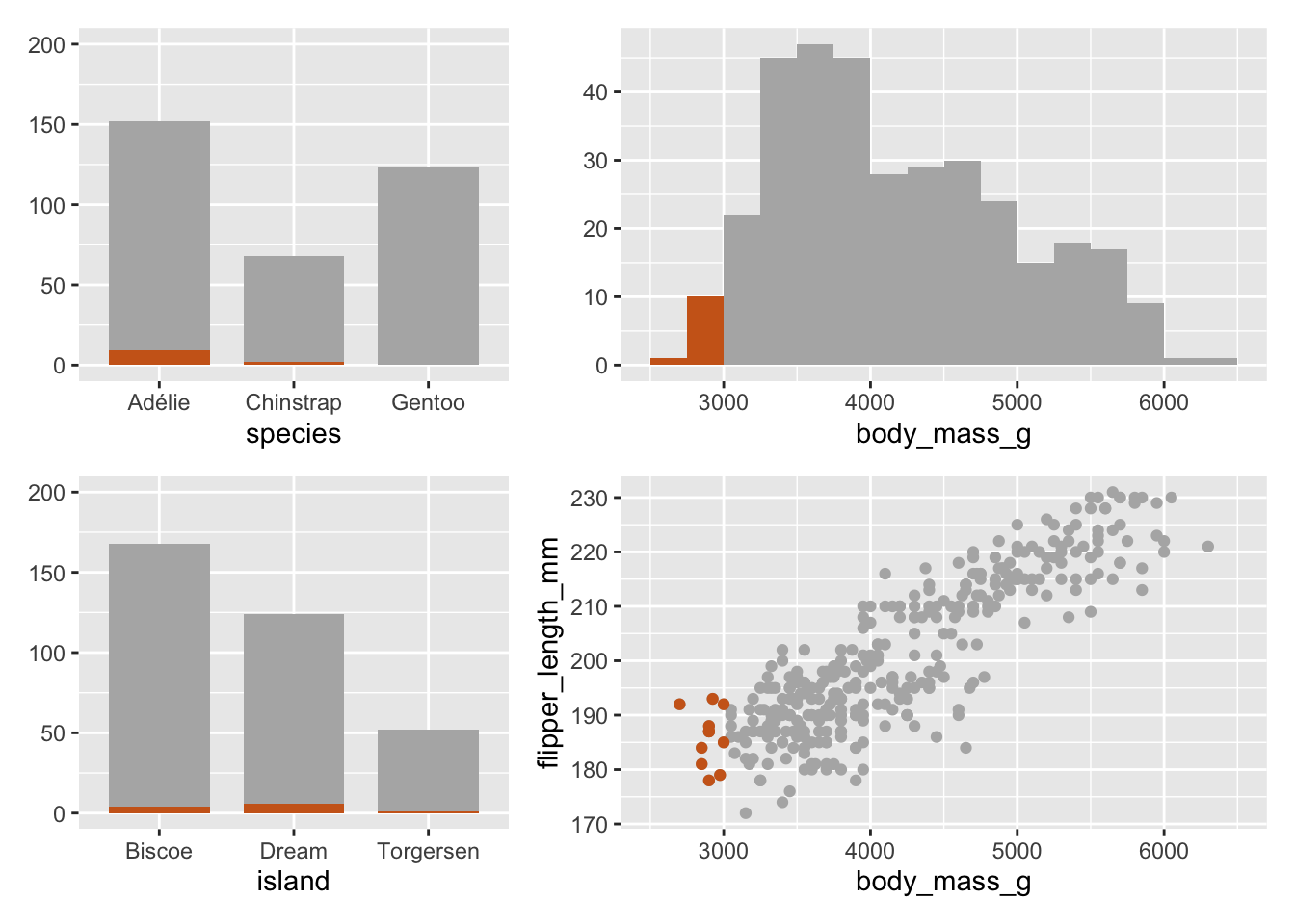
Figure 18.4: Penguins weighing no more than 3 kg highlighted in all plots

At this stage, it could be worth investigating what values these subsets have for other variables. This could be done by drawing the additional plots with the appropriate subset layer. Figure 18.5 shows boxplots for bill length and depth with the lightest penguins drawn in separate boxplots in brown beside boxplots for the rest of the data. With two exceptions, the light penguins have shorter bills than most other penguins. Their bill depths are about the same.

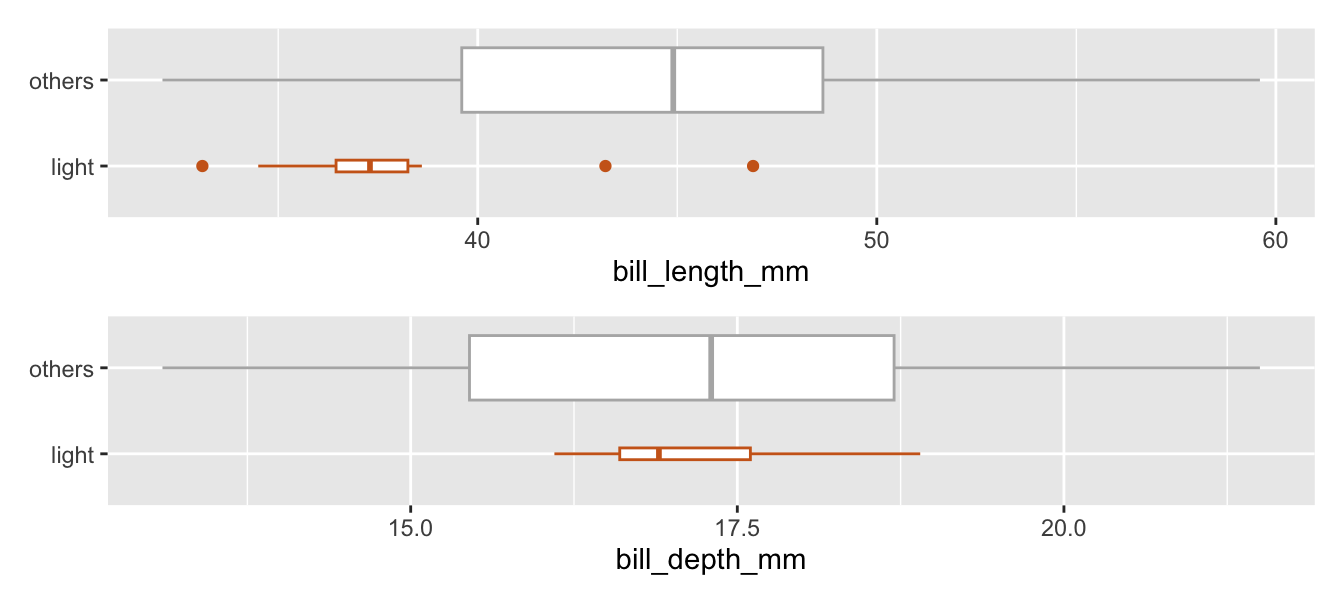
Figure 18.5: Penguins weighing no more than 3 kg plotted beside the rest, comparing bill lengths and bill depths

The boxplots have been drawn with widths proportional to the square roots of the numbers in the groups (331 and 11). The effect may be dramatic, but it emphasises how small the selected group is. By contrast consider boxplots of the same two bill measurements comparing Dream Island penguins to the rest. Bill lengths are about the same, while bill depths are larger.

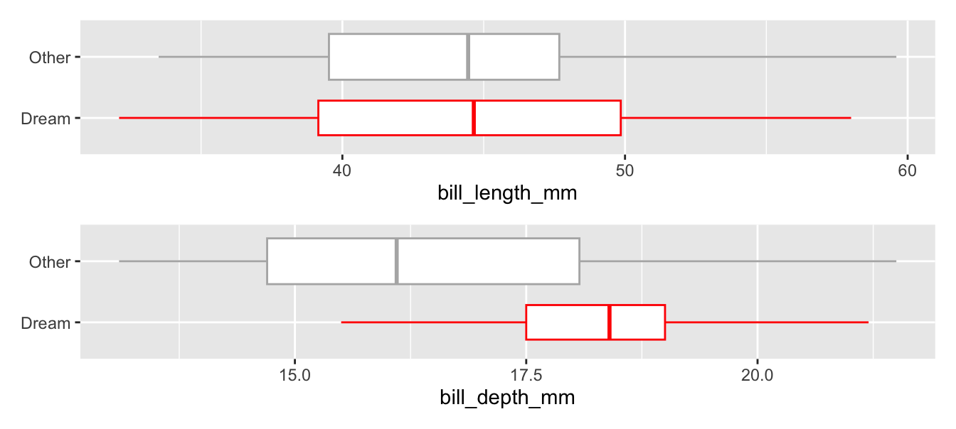
Figure 18.6: Dream Island penguins plotted beside the rest, comparing bill lengths and bill depths

Highlighting like this is a basic tool in interactive graphics where you select cases in one plot and they are then immediately highlighted in all other plots. Static versions, ghostplots, do not offer the same immediacy and flexibility, but can be drawn by creating a subset of just the selected cases. The plots required are drawn with the full dataset, using a muted colouring, and an additional layer is added to each plot using the subset. The selected objects are coloured more strongly, for instance in red or blue.