24.1 Vehicle accidents involving deer

Bavarian data of the numbers of vehicle accidents involving deer over the full ten years from 2002 to 2011 have been modelled in depth in Hothorn et al. (2015). The data were also used in Hothorn (2020) and are available in the supplementary material on the publishing journal’s website.

Figure 24.1 shows a smoothed version of the daily number of vehicle accidents involving deer. There was an increase of around 50% over the ten years.

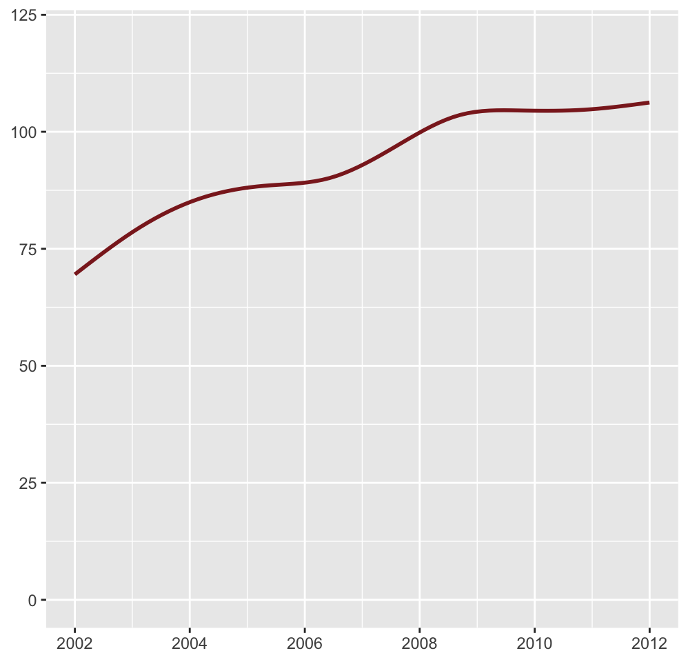
Figure 24.1: Smoothed numbers of deer-vehicle accidents per day in Bavaria over ten years from Jan 1st 2002 to Dec 31st 2011

In Figure 24.1, and in all the plots in this chapter, the time axis labels are placed at the start of the labelled period.

Figure 24.2 shows an initial plot to explore monthly seasonality. Each panel of the plot displays the aggregate data from that month for each year and the average for the month over the whole time series in blue. Here the data are per month, which is the why the vertical scale is so different to that in Figure 24.1.

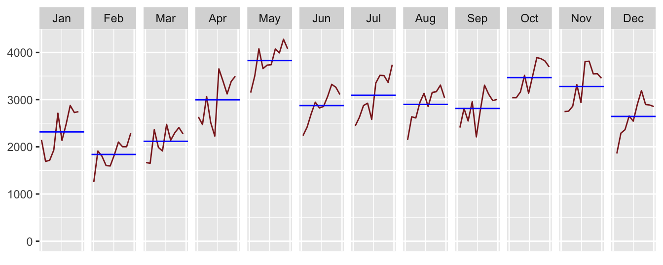
Figure 24.2: Monthly numbers of deer-vehicle accidents across the ten years 2002 to 2011.

There is an overall rise in each monthly series with some, occasionally dramatic, variation, and a possible seasonal pattern. Summarising over months is a bit of an approximation, as the months are not all the same length. An alternative is to fit another smooth across the data, rougher than the one in Figure 24.1, and overlay the resulting individual annual series. This has been done in Figure 24.3. An adaptive smooth has been used.

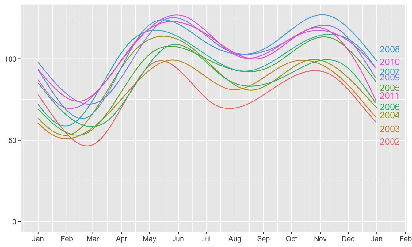
Figure 24.3: Numbers of deer-vehicle accidents across all ten years overlaid from Jan 1st to Dec 31st

The plot shows a fairly regular pattern across the years with peaks in May-June and October-November and lower values in Spring and, to a lesser extent, Summer. The highest numbers are about double the lowest ones.

Given the differences in vehicle traffic between weekdays and weekends and public holidays, there could well be weekly patterns as well. An initial analysis, without treating public holidays as similar to weekends is shown in Figure 24.4.

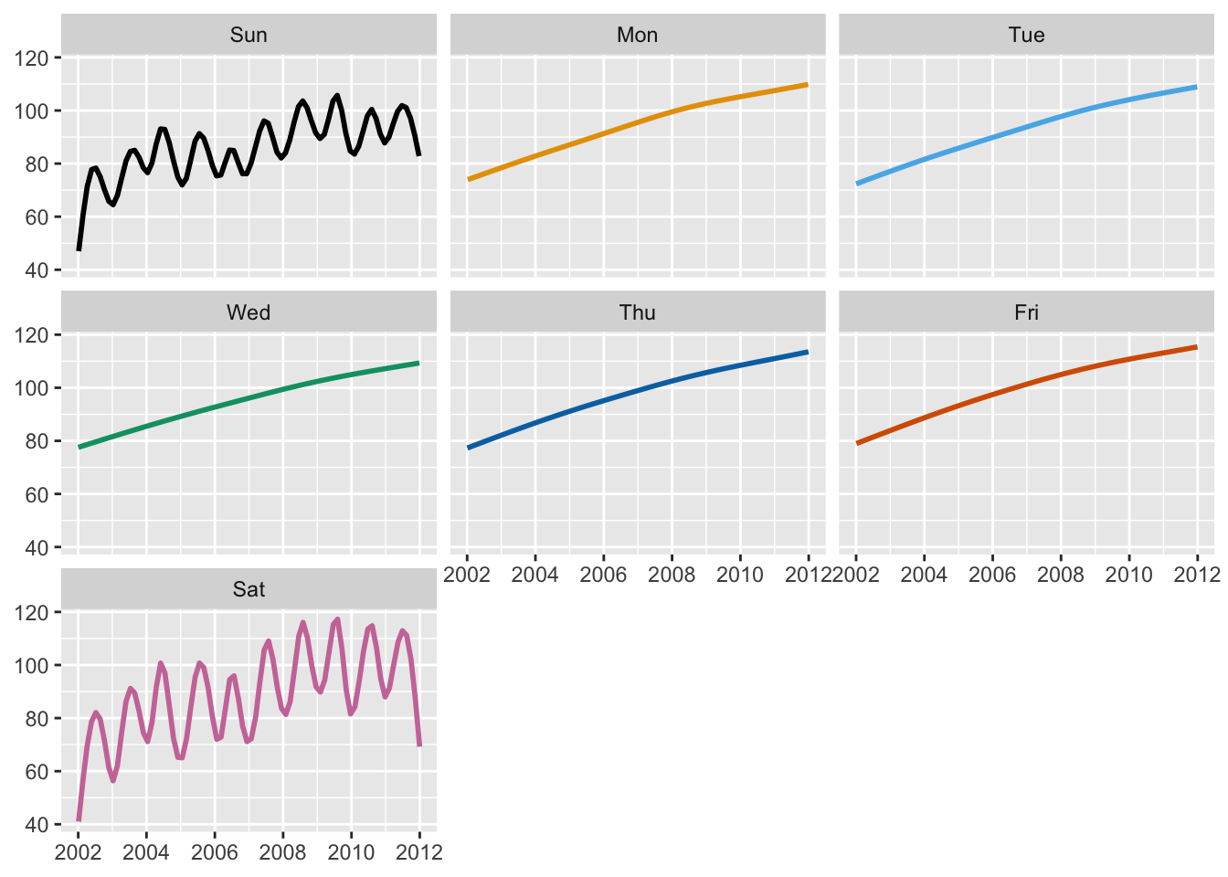
Figure 24.4: Day of the week patterns in numbers of deer-vehicle accidents

A few values of the smoothing parameter were tried and the rounded value leading to this display was chosen, as it suggested a clear differentiation between weekdays and weekends. The peaks in summer and the troughs in winter stand out. Presumably there is less vehicle traffic at weekends in winter and hence fewer accidents with deer then than in summer. The lack of seasonality in the weekday plots offers supporting evidence.

In the early days of time series analysis there were suggestions that time series could be decomposed into components of trend, seasonality, and noise. Sometimes this works well, sometimes it is difficult to disentangle trend and seasonality. That is to some extent the case here.

The data available are more detailed than these graphics imply. Numbers of accidents are reported for every half-hour of every day, i.e. there are 48 numbers per day. Figures 24.5 and 24.6 investigate the monthly averages of these daily data across months by year and across years by month. Unsurprisingly there are differences in the patterns by years, as the data are shifted for the individual months. This is easier to see in Figure 24.6, where the two peaks are further apart for the summer months and closer together for the winter months. According to Hothorn et al. (2015) the deer are on the move more around sunrise and after sunset, which explains these peaks and their pattern across the year. In that paper, heat maps were used to display the daily data.

Figures 24.5 and 24.6 are a good example of where the choice of which time variable to facet by is important. Both plots convey the information, but the second one does it better.

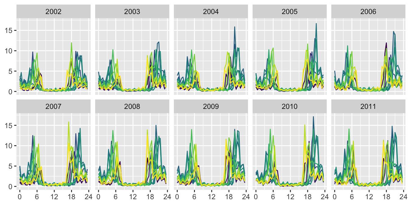
Figure 24.5: Average daily patterns in numbers of deer-vehicle accidents by month (the coloured lines) and year

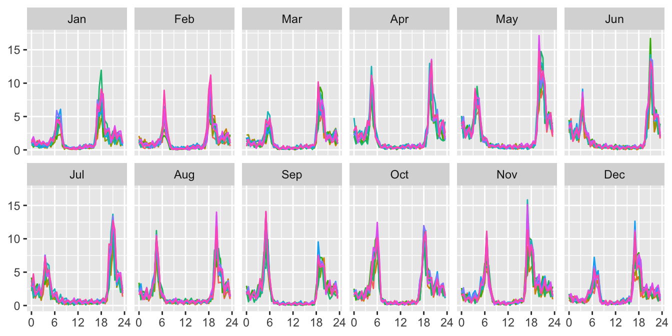
Figure 24.6: Daily patterns in numbers of deer-vehicle accidents by month across the years (the coloured lines)