29.1 MatchIt
Procedure typically involves (proposed by Noah Freifer using MatchIt)
- planning
- matching
- checking (balance)
- estimating the treatment effect
examine treat on re78
- Planning
select type of effect to be estimated (e.g., mediation effect, conditional effect, marginal effect)
select the target population
select variables to match/balance (Austin 2011) (T. J. VanderWeele 2019)
- Check Initial Imbalance
# No matching; constructing a pre-match matchit object
m.out0 <- matchit(
    formula(treat ~ age + educ + race
            + married + nodegree + re74 + re75, env = lalonde),
    data = data.frame(lalonde),
    method = NULL,
    # assess balance before matching
    distance = "glm" # logistic regression
)

# Checking balance prior to matching
summary(m.out0)- Matching
# 1:1 NN PS matching w/o replacement
m.out1 <- matchit(treat ~ age + educ,
                  data = lalonde,
                  method = "nearest",
                  distance = "glm")
m.out1
#> A matchit object
#>  - method: 1:1 nearest neighbor matching without replacement
#>  - distance: Propensity score
#>              - estimated with logistic regression
#>  - number of obs.: 614 (original), 370 (matched)
#>  - target estimand: ATT
#> - covariates: age, educ- Check balance
Sometimes you have to make trade-off between balance and sample size.
# Checking balance after NN matching
summary(m.out1, un = FALSE)
#>
#> Call:
#> matchit(formula = treat ~ age + educ, data = lalonde, method = "nearest",
#>     distance = "glm")
#>
#> Summary of Balance for Matched Data:
#>          Means Treated Means Control Std. Mean Diff. Var. Ratio eCDF Mean
#> distance        0.3080        0.3077          0.0094     0.9963    0.0033
#> age            25.8162       25.8649         -0.0068     1.0300    0.0050
#> educ           10.3459       10.2865          0.0296     0.5886    0.0253
#>          eCDF Max Std. Pair Dist.
#> distance   0.0432          0.0146
#> age        0.0162          0.0597
#> educ       0.1189          0.8146
#>
#> Sample Sizes:
#>           Control Treated
#> All           429     185
#> Matched       185     185
#> Unmatched     244       0
#> Discarded       0       0

# examine visually
plot(m.out1, type = "jitter", interactive = FALSE)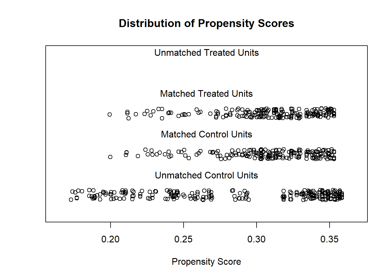
Try Full Match (i.e., every treated matches with one control, and every control with one treated).
# Full matching on a probit PS
m.out2 <- matchit(treat ~ age + educ,
                  data = lalonde,
                  method = "full",
                  distance = "glm",
                  link = "probit")
m.out2
#> A matchit object
#>  - method: Optimal full matching
#>  - distance: Propensity score
#>              - estimated with probit regression
#>  - number of obs.: 614 (original), 614 (matched)
#>  - target estimand: ATT
#>  - covariates: age, educ
Checking balance again
# Checking balance after full matching
summary(m.out2, un = FALSE)
#>
#> Call:
#> matchit(formula = treat ~ age + educ, data = lalonde, method = "full",
#>     distance = "glm", link = "probit")
#>
#> Summary of Balance for Matched Data:
#>          Means Treated Means Control Std. Mean Diff. Var. Ratio eCDF Mean
#> distance        0.3082        0.3081          0.0023     0.9815    0.0028
#> age            25.8162       25.8035          0.0018     0.9825    0.0062
#> educ           10.3459       10.2315          0.0569     0.4390    0.0481
#>          eCDF Max Std. Pair Dist.
#> distance   0.0270          0.0382
#> age        0.0249          0.1110
#> educ       0.1300          0.9805
#>
#> Sample Sizes:
#>               Control Treated
#> All            429.       185
#> Matched (ESS)  145.23     185
#> Matched        429.       185
#> Unmatched        0.         0
#> Discarded        0.         0

plot(summary(m.out2))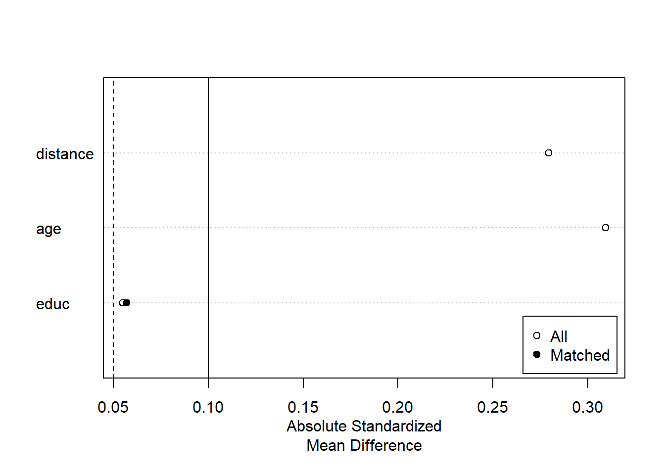
Exact Matching
# Full matching on a probit PS
m.out3 <-
    matchit(
        treat ~ age + educ,
        data = lalonde,
        method = "exact"
    )
m.out3
#> A matchit object
#>  - method: Exact matching
#>  - number of obs.: 614 (original), 332 (matched)
#>  - target estimand: ATT
#>  - covariates: age, educ
Subclassfication
m.out4 <- matchit(
    treat ~ age + educ,
    data = lalonde,
    method = "subclass"
)
m.out4
#> A matchit object
#>  - method: Subclassification (6 subclasses)
#>  - distance: Propensity score
#>              - estimated with logistic regression
#>  - number of obs.: 614 (original), 614 (matched)
#>  - target estimand: ATT
#>  - covariates: age, educ

# Or you can use in conjunction with "nearest"
m.out4 <- matchit(
    treat ~ age + educ,
    data = lalonde,
    method = "nearest",
    option = "subclass"
)
m.out4
#> A matchit object
#>  - method: 1:1 nearest neighbor matching without replacement
#>  - distance: Propensity score
#>              - estimated with logistic regression
#>  - number of obs.: 614 (original), 370 (matched)
#>  - target estimand: ATT
#>  - covariates: age, educ
Optimal Matching
m.out5 <- matchit(
    treat ~ age + educ,
    data = lalonde,
    method = "optimal",
    ratio = 2
)
m.out5
#> A matchit object
#>  - method: 2:1 optimal pair matching
#>  - distance: Propensity score
#>              - estimated with logistic regression
#>  - number of obs.: 614 (original), 555 (matched)
#>  - target estimand: ATT
#>  - covariates: age, educ
Genetic Matching
m.out6 <- matchit(
    treat ~ age + educ,
    data = lalonde,
    method = "genetic"
)
m.out6
#> A matchit object
#>  - method: 1:1 genetic matching without replacement
#>  - distance: Propensity score
#>              - estimated with logistic regression
#>  - number of obs.: 614 (original), 370 (matched)
#>  - target estimand: ATT
#> - covariates: age, educ- Estimating the Treatment Effect
# get matched data
m.data1 <- match.data(m.out1)

head(m.data1)
#>      treat age educ   race married nodegree re74 re75       re78  distance
#> NSW1     1  37   11  black       1        1    0    0  9930.0460 0.2536942
#> NSW2     1  22    9 hispan       0        1    0    0  3595.8940 0.3245468
#> NSW3     1  30   12  black       0        0    0    0 24909.4500 0.2881139
#> NSW4     1  27   11  black       0        1    0    0  7506.1460 0.3016672
#> NSW5     1  33    8  black       0        1    0    0   289.7899 0.2683025
#> NSW6     1  22    9  black       0        1    0    0  4056.4940 0.3245468
#>      weights subclass
#> NSW1       1        1
#> NSW2       1       98
#> NSW3       1      109
#> NSW4       1      120
#> NSW5       1      131
#> NSW6 1 142library("lmtest") #coeftest
library("sandwich") #vcovCL
# imbalance matched dataset
fit1 <- lm(re78 ~ treat + age + educ ,
data = m.data1,
weights = weights)
coeftest(fit1, vcov. = vcovCL, cluster = ~subclass)
#>
#> t test of coefficients:
#>
#> Estimate Std. Error t value Pr(>|t|)
#> (Intercept) -174.902 2445.013 -0.0715 0.943012
#> treat -1139.085 780.399 -1.4596 0.145253
#> age 153.133 55.317 2.7683 0.005922 **
#> educ 358.577 163.860 2.1883 0.029278 *
#> ---
#> Signif. codes: 0 '***' 0.001 '**' 0.01 '*' 0.05 '.' 0.1 ' ' 1treat coefficient = estimated ATT
# balance matched dataset
m.data2 <- match.data(m.out2)

fit2 <- lm(re78 ~ treat + age + educ ,
           data = m.data2, weights = weights)

coeftest(fit2, vcov. = vcovCL, cluster = ~subclass)
#>
#> t test of coefficients:
#>
#>             Estimate Std. Error t value Pr(>|t|)
#> (Intercept) 2151.952   3141.152  0.6851  0.49355
#> treat       -725.184    703.297 -1.0311  0.30289
#> age          120.260     53.933  2.2298  0.02612 *
#> educ         175.693    241.694  0.7269  0.46755
#> ---
#> Signif. codes:  0 '***' 0.001 '**' 0.01 '*' 0.05 '.' 0.1 ' ' 1
When reporting, remember to mention
- the matching specification (method, and additional options)
- the distance measure (e.g., propensity score)
- other methods, and rationale for the final chosen method.
- balance statistics of the matched dataset.
- number of matched, unmatched, discarded
- estimation method for treatment effect.
References
Austin, Peter C. 2011. “Optimal Caliper Widths for Propensity-Score Matching When Estimating Differences in Means and Differences in Proportions in Observational Studies.” Pharmaceutical Statistics 10 (2): 150–61.
VanderWeele, Tyler J. 2019. “Principles of Confounder Selection.” European Journal of Epidemiology 34: 211–19.