3.6 Prior information
All the estimators thus far surveyed in this chapter are based purely on the \(T\) historical data points \(\bm{x}_1,\dots,\bm{x}_T\). Unfortunately, in many practical settings, as discussed in Section 3.2, the number of observations is not large enough to achieve a proper estimation of the model parameters with a sufficiently small error. Researchers and practitioners have spent decades trying to deal with this issue and devising a variety of mechanisms to improve the estimators. The basic recipe is to somehow incorporate any prior information that one may have available. We will next overview three notable ways to incorporate prior information into the parameter estimation process:
- shrinkage: to incorporate prior knowledge on the parameters in the form of targets;
- factor modeling: to incorporate structural information; and
- Black-Litterman: to combine the data with discretionary views.
Each of these approaches deserves a whole chapter—if not a whole book—but we will merely scratch the tip of the iceberg here, while providing key references to probe further for the interested reader.
3.6.1 Shrinkage
Shrinkage is a popular technique to reduce the estimation error by introducing a bias in the estimator. In statistics, this idea goes back to 1955 with Stein’s seminal publication (Stein, 1955). In the financial area, it was popularized by its application to shrinkage in the covariance matrix in the early 2000s (Ledoit and Wolf, 2004) and it is now covered in many textbooks (Meucci, 2005) and surveys (Bun et al., 2017).
The mean squared error (MSE) of an estimator can be separated into two terms: the bias and the variance. This is a basic concept in estimation theory referred to as the bias-variance trade-off (Kay, 1993; Scharf, 1991). Mathematically, for a given parameter \(\bm{\theta}\) and an estimator \(\hat{\bm{\theta}}\), the bias-variance trade-off reads: \[ \begin{aligned} \textm{MSE}(\hat{\bm{\theta}}) & \triangleq \E\left[\big\|\hat{\bm{\theta}} - \bm{\theta}\big\|^2\right]\\ & = \E\left[\big\|\hat{\bm{\theta}} - \E\big[\hat{\bm{\theta}}\big]\big\|^2\right] + \big\|\E\big[\hat{\bm{\theta}}\big] - \bm{\theta}\big\|^2\\ & = \textm{Var}\big(\hat{\bm{\theta}}\big) + \textm{Bias}^2\big(\hat{\bm{\theta}}\big). \end{aligned} \]
In the small sample regime (i.e., when the number of observations is small), the main source of error comes from the variance of the estimator (since the estimator is based on a small number of random samples). In the large sample regime, on the other hand, one may expect the variance of the estimator to be reduced and the bias to dominate the overall error.
Traditionally, unbiased estimators had always been desirable. To the surprise of the statistical community, Stein proved in 1955 in a seminar paper (Stein, 1955) that it might be advantageous to allow for some bias in order to achieve a smaller overall error. This can be implemented by shrinking the estimator to some known target value. Mathematically, for a given estimator \(\hat{\bm{\theta}}\) and some target \(\bm{\theta}^\textm{tgt}\) (i.e., the prior information), a shrinkage estimator is given by \[ \hat{\bm{\theta}}^\textm{sh} = (1 - \rho)\, \hat{\bm{\theta}} + \rho\, \bm{\theta}^\textm{tgt}, \] where \(\rho\) (with \(0 \le \rho \le 1\)) is the shrinkage trade-off parameter or shrinkage factor.
In practice, there are two important issues when implementing shrinkage:
The choice of the target \(\bm{\theta}^\textm{tgt}\), which represents the prior information and, in a financial context, may come from discretionary views on the market.
The choice of the shrinkage factor \(\rho\), which may look like a trivial problem, but the reality is that tons of ink have been devoted to this topic in the literature.
While the choice of the target is important, it is perhaps surprising that the most critical part is the choice of the shrinkage factor \(\rho\). The reason is that, no matter how poorly chosen the target is, a proper choice of the shrinkage factor can always weight the target in the right amount. There are two main philosophies when it comes to choosing the shrinkage factor \(\rho\):
- empirical choice based on cross-validation, and
- analytical choice based on sophisticated mathematics.
In our context of financial data, the parameter \(\bm{\theta}\) may represent the mean vector \(\bmu\) or the covariance matrix \(\bSigma\), and the estimator \(\hat{\bm{\theta}}\) may be, for example, the sample mean or the sample covariance matrix.
Shrinking the mean vector
Consider the mean vector \(\bmu\) and the sample mean estimator in (3.2): \[ \hat{\bmu} = \frac{1}{T}\sum_{t=1}^{T}\bm{x}_{t}. \] As we know from Section 3.2, the sample mean \(\hat{\bmu}\) is an unbiased estimator, \(\E\left[\hat{\bmu}\right] = \bmu\). In addition, from the central limit theorem, we can further characterize its distribution as \[ \hat{\bmu} \sim \mathcal{N}\left(\bmu,\frac{1}{T}\bSigma\right) \] and its MSE as \[ \E\left[\big\|\hat{\bmu} - \bmu\big\|^2\right] = \frac{1}{T}\textm{Tr}(\bSigma). \]
A startling result proved by Stein in 1955 in a seminal paper (Stein, 1955) is that, in terms of MSE, this approach is suboptimal and it is better to allow some bias in order to reduce the overall MSE, which can be achieved in the form of shrinkage.
The so-called James-Stein estimator (W. James and Stein, 1961) is \[ \hat{\bmu}^\textm{JS} = (1 - \rho)\, \hat{\bmu} + \rho\, \bmu^\textm{tgt}, \] where \(\bmu^\textm{tgt}\) is the target and \(\rho\) the shrinkage factor. To be precise, regardless of the chosen target \(\bmu^\textm{tgt}\), one can always improve the MSE, \[ \E\left[\big\|\hat{\bmu}^\textm{JS} - \bmu\big\|^2\right] \leq \E\left[\big\|\hat{\bmu} - \bmu\big\|^2\right], \] with a properly chosen \(\rho\), such as (Jorion, 1986) \[ \rho = \frac{(N+2)}{(N+2) + T\times\left(\hat{\bmu} - \bmu^\textm{tgt}\right)^\T\bSigma^{-1}\left(\hat{\bmu} - \bmu^\textm{tgt}\right)}, \] where, in practice, \(\bSigma\) can be replaced by an estimation \(\hat{\bSigma}\). The choice of \(\rho\) was also considered under heavy-tailed distributions in (Srivastava and Bilodeau, 1989).
It is worth emphasizing that this result holds regardless of the choice of the target \(\bmu^\textm{tgt}\). In other words, one can choose the target as bad as desired, but still the MSE can be reduced (phenomenon often referred to as the Stein paradox). This happens because the value of \(\rho\) automatically adapts in the following ways:
- \(\rho \rightarrow 0\) as \(T\) increases, i.e., the more observations, the stronger the belief on the original sample mean estimator;
- \(\rho \rightarrow 0\) as the target disagrees with the sample mean (built-in safety mechanism under wrongly chosen targets).
While it is true that the MSE can be reduced no matter the choice of the target, the size of the improvement will obviously depend on how good and informative the target is. Any available prior information can be incorporated in the target. Some reasonable and common choices are (Jorion, 1986):
- zero: \(\bmu^\textm{tgt} = \bm{0}\);
- grand mean: \(\bmu^\textm{tgt} = \frac{\bm{1}^\T\hat{\bmu}}{N}\times\bm{1}\); and
- volatility-weighted grand mean: \(\bmu^\textm{tgt} = \frac{\bm{1}^\T\hat{\bSigma}^{-1}\hat{\bmu}}{\bm{1}^\T\hat{\bSigma}^{-1}\bm{1}}\times\bm{1}\).
Shrinking the covariance matrix
Consider the covariance matrix \(\bSigma\) and the sample covariance matrix estimator in (3.3): \[ \hat{\bSigma} = \frac{1}{T-1}\sum_{t=1}^{T}(\bm{x}_t - \hat{\bmu})(\bm{x}_t - \hat{\bmu})^\T. \] As we know from Section 3.2, the sample covariance matrix \(\hat{\bSigma}\) is an unbiased estimator, \(\E\big[\hat{\bSigma}\big] = \bSigma\). We will now introduce some bias in the form of shrinkage.
The shrinkage estimator for the covariance matrix has the form: \[ \hat{\bSigma}^\textm{sh} = (1 - \rho)\, \hat{\bSigma} + \rho\, \bSigma^\textm{tgt}, \] where \(\bSigma^\textm{tgt}\) is the target and \(\rho\) the shrinkage factor.
The idea of shrinkage of the covariance matrix had been already used in the 1980s, for example, in wireless communications systems under the term “diagonal loading” (Abramovich, 1981). In finance, it was popularized in the early 2000s (Ledoit and Wolf, 2003, 2004) and more mature tools developed in the last two decades (Bun et al., 2017).
Common choices for the covariance matrix target are:
- scaled identity: \(\bSigma^\textm{tgt} = \frac{1}{N}\textm{Tr}\big(\hat{\bSigma}\big)\times\bm{I}\);
- diagonal matrix: \(\bSigma^\textm{tgt} = \textm{Diag}\big(\hat{\bSigma}\big)\), which is equivalent to using the identity matrix as the correlation matrix target, i.e., \(\bm{C}^\textm{tgt} = \bm{I}\); and
- equal-correlation matrix: \(\bm{C}^\textm{tgt}\) with off-diagonal elements all equal to the average cross-correlation of assets.
The shrinkage factor \(\rho\) can be determined empirically via cross-validation or analytically via a mathematically sophisticated approach such as random matrix theory (RMT) (Bun et al., 2006, 2017). This was made popular in the financial community by Ledoit and Wolf in the early 2000s (Ledoit and Wolf, 2003, 2004). The idea is simple: choose \(\rho\) to form the shrinkage estimator \(\hat{\bSigma}^\textm{sh}\) in order to minimize the error measure \(\E\left[\big\|\hat{\bSigma}^\textm{sh} - \bSigma\big\|_\textm{F}^2\right]\). Of course, this problem is ill-posed since precisely the true covariance matrix \(\bSigma\) is unknown; otherwise, the so-called “oracle” solution is obtained as \[ \rho = \frac{\E\left[\big\|\hat{\bSigma} - \bSigma\big\|_\textm{F}^2\right]}{\E\left[\big\|\hat{\bSigma} - \bSigma^\textm{tgt}\big\|_\textm{F}^2\right]}. \] This is where the magic of RMT truly shines: asymptotically for large \(T\) and \(N\), one can derive a consistent estimator that does not require knowledge of \(\bSigma\) as \[\begin{equation} \rho = \textm{min}\left(1, \frac{\frac{1}{T}\sum_{t=1}^T \big\|\hat{\bSigma} - \bm{x}_t\bm{x}_t^\T\big\|_\textm{F}^2}{\big\|\hat{\bSigma} - \bSigma^\textm{tgt}\big\|_\textm{F}^2}\right). \tag{3.11} \end{equation}\] The usefulness of RMT is that the results are extremely good even when \(T\) and \(N\) are not very large, i.e., the asymptotics kick in very fast in practice.
One important way to extend shrinkage is to consider heavy-tailed distributions (introduced in Section 3.5) and derive an appropriate choice for \(\rho\) under heavy tails (Y. Chen et al., 2011; Ollila et al., 2023, 2021; Ollila and Raninen, 2019).
It is worth pointing out that the shrinkage factor in (3.11) is derived to minimize the error measure \(\E\left[\big\|\hat{\bSigma}^\textm{sh} - \bSigma\big\|_\textm{F}^2\right]\). Alternatively, one can consider more meaningful measures of error better suited to the purpose of portfolio design, with the drawback that the mathematical derivation of \(\rho\) becomes more involved and cannot be obtained in a nice closed-form expression such as (3.11). Some examples include the following (cf. (Feng and Palomar, 2016)):
Portfolios designed based on \(\bSigma\) are more directly related to the inverse covariance matrix \(\bSigma^{-1}\) (see Chapter 7). Thus, it makes sense to measure the error in terms of the inverse covariance matrix instead \(\E\left[\big\|\big(\hat{\bSigma}^\textm{sh}\big)^{-1} - \bSigma^{-1}\big\|_\textm{F}^2\right]\) (M. Zhang, Rubio, and Palomar, 2013).
Portfolios are typically evaluated in terms of the Sharpe ratio, which is related to the term \(\bSigma^{-1}\bmu\) (see Chapter 7). Thus, it has more practical meaning to choose \(\rho\) to maximize the achieved Sharpe ratio (Ledoit and Wolf, 2017; M. Zhang, Rubio, Palomar, and Mestre, 2013).
The covariance shrinkage estimator is a linear combination of the estimate \(\hat{\bSigma}\) and the target \(\bSigma^\textm{tgt}\). Another way to extend this idea is to consider a nonlinear shrinkage in terms of eigenvalues of the covariance matrix, which again leads to an increased sophistication in the required mathematics, e.g., (Ledoit and Wolf, 2017), (Bun et al., 2006, 2017), (Bartz, 2016), and (Tyler and Yi, 2020).
Numerical experiments
Figure 3.13 shows the estimation error of shrinkage estimators as a function of the number of observations \(T\) for synthetic Gaussian data. We can observe that a clear improvement is achieved in the estimation of the mean vector, whereas only a modest improvement is achieved in the estimation of the covariance matrix. As expected, the benefit of shrinkage diminishes as the number of observations grows large.
Interestingly, the shrinkage to zero seems to produce the best results. This is not unexpected since, according to the efficient-market hypothesis (Fama, 1970), the prices are expected to contain all the current information of the assets (including future prospects). Thus, a reasonable forecast for the prices are just the current prices or, equivalently in terms of returns, the zero return vector.
It is important to emphasize that these numerical results are obtained in terms of the mean squared error of the estimators. However, in the context of portfolio optimization, the mean squared error may not be the best measure of errors. Thus, these results should be taken with a grain of salt and more appropriate measures of error should probably be considered (Ledoit and Wolf, 2017).
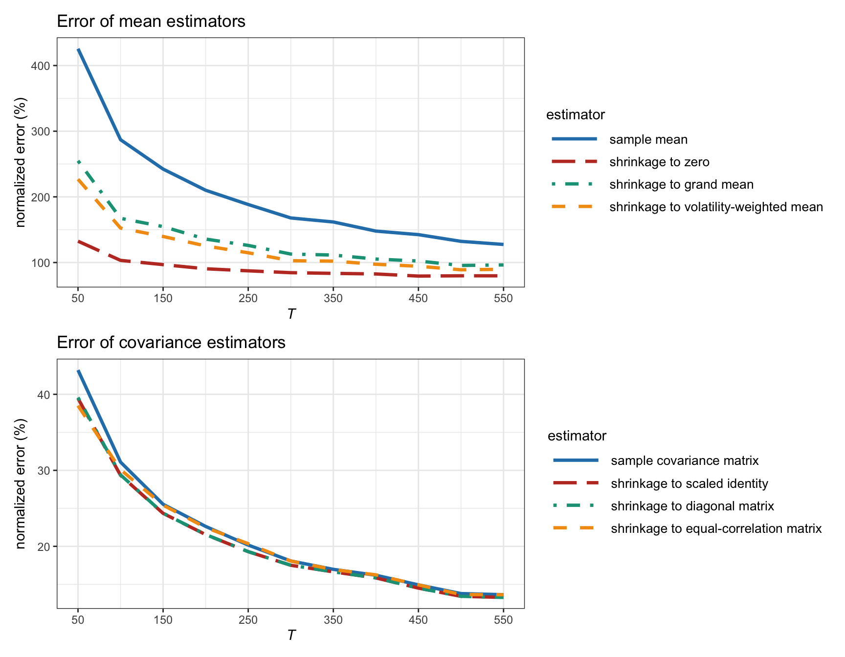
Figure 3.13: Estimation error of different shrinkage estimators versus number of observations (for Gaussian data with \(N=100\)).
3.6.2 Factor models
Factor modeling is standard material in finance and can be found in many textbooks, such as (Campbell et al., 1997; Fabozzi et al., 2010; Lütkepohl, 2007; Ruppert and Matteson, 2015; Tsay, 2010, 2013).
The idea is to introduce prior information into the basic i.i.d. model of the returns in (3.1), \(\bm{x}_t = \bmu + \bm{\epsilon}_t\), in the form of a more sophisticated asset structure. For example, the simplest case is the single-factor model: \[\begin{equation} \bm{x}_t = \bm{\alpha} + \bm{\beta} f^\textm{mkt}_t + \bm{\epsilon}_t, \tag{3.12} \end{equation}\] where \(\bm{\alpha}\in\R^N\) and \(\bm{\beta}\in\R^N\) are the so-called “alpha” and “beta” of the \(N\) assets, respectively, the scalar \(f^\textm{mkt}_t\) is the market factor (or market index), and \(\bm{\epsilon}_t\) is the zero-mean residual component. The “beta” refers to how sensitive the asset is to the overall market, whereas the “alpha” indicates the excess return of the asset. As explored in Chapter 6, one common constraint in portfolio design is to be market-neutral, which refers precisely to the portfolio being orthogonal to \(\bm{\beta}\).
The single-factor model in (3.12) has some connection with the capital asset pricing model (CAPM) introduced by Sharpe in (Sharpe, 1964). In particular, the CAPM is concerned with the expected excess returns and assumes a zero “alpha”: \[\begin{equation} \E[x_i] - r_f = \beta_i \left(\E\left[f^\textm{mkt}]\right] - r_f\right), \tag{3.13} \end{equation}\] where \(r_f\) denotes the risk-free asset return.
More generally, the multi-factor modeling is \[\begin{equation} \bm{x}_t = \bm{\alpha} + \bm{B} \bm{f}_t + \bm{\epsilon}_t, \tag{3.14} \end{equation}\] where now \(\bm{f}_t\in\R^K\) contains \(K\) factors (also termed risk factors)—typically with \(K\ll N\)—and the matrix \(\bm{B}\in\R^{N\times K}\) contains along its columns the betas (also called factor loadings) for each of the factors. It is also possibly to include time-dependency in the factors, leading to the so-called dynamic factor models (Fabozzi et al., 2010).
The residual term \(\bm{\epsilon}_t\) in (3.12) and (3.14)—typically referred to as the idiosyncratic component—is assumed to have independent elements or, in other words, a diagonal covariance matrix \(\bm{\Psi} = \textm{Diag}(\psi_1, \dots, \psi_N)\in\R^{N\times N}\). The rationale is that the correlation among the assets is already modeled by the other term via the factors.
One key realization in factor modeling is that the number of parameters of the model to be estimated is significantly reduced. For example, in the case of \(N=500\) assets and \(K=3\) factors, the number of parameters in the plain i.i.d. model in (3.1) is 125,750 (\(N\) for \(\bmu\) and \(N(N + 1)/2\) for the symmetric covariance matrix \(\bSigma\)), whereas for the factor model in (3.14) the number of parameters is 2,500 (\(N\) for \(\bm{\alpha}\), \(NK\) for \(\bm{B}\), and \(N\) for the diagonal covariance matrix \(\bm{\Psi}\)).
The mean and covariance matrix according to the model (3.14) are given by \[\begin{equation} \begin{aligned} \bmu &= \bm{\alpha} + \bm{B} \bmu_f\\ \bSigma &= \bm{B} \bSigma_f \bm{B}^\T + \bm{\Psi}, \end{aligned} \tag{3.15} \end{equation}\] where \(\bmu_f\) and \(\bSigma_f\) are the mean vector and covariance matrix, respectively, of the factors \(\bm{f}_t\). Observe that the covariance matrix has effectively been decomposed into a low-rank component \(\bm{B} \bSigma_f \bm{B}^\T\) (with rank \(K\)) and a full-rank diagonal component \(\bm{\Psi}\).
Essentially, factor models decompose the asset returns into two parts: the low-dimensional factor component, \(\bm{B} \bm{f}_t\), and the idiosyncratic residual noise \(\bm{\epsilon}_t\). Depending on the assumptions made on the factors \(\bm{f}_t\) and “betas” in \(\bm{B}\), factor models can be classified into three types:
Macroeconomic factor models: Factors are observable economic and financial time series but the loading matrix \(\bm{B}\) is unknown.
Fundamental factor models: Some models construct the loading matrix \(\bm{B}\) from asset characteristics with unknown factors, whereas others construct the factors from asset characteristics first.
Statistical factor models: Both the factors and the loading matrix \(\bm{B}\) are unknown.
Macroeconomic factor models
In macroeconomic factor models, the factors are observable time series such as the market index, the growth rate of the GDP13, interest rate, inflation rate, etc. In the investment world, factors are computed in complicated proprietary ways from a variety of non-accessible sources of data and, typically, investment funds pay a substantial premium to have access to them. Such expensive factors are not available to small investors, which have to rely on readily available sources of data.
Given the factors, the estimation of the model parameters can be easily formulated as a simple least squares regression problem: \[ \begin{array}{ll} \underset{\bm{\alpha},\bm{B}}{\textm{minimize}} & \begin{aligned}[t] \sum_{t=1}^{T} \left\Vert \bm{x}_t - \left(\bm{\alpha} + \bm{B} \bm{f}_t \right)\right\Vert_2^2\end{aligned}, \end{array} \] from which \(\bmu\) and \(\bSigma\) can then be obtained from (3.15).
Fundamental factor models
Fundamental factor models use observable asset specific characteristics (termed fundamentals), such as industry classification, market capitalization, style classification (e.g., value, growth), to determine the factors. Typically, two approaches are followed in the industry:
Fama-French approach: First, a portfolio is formed based on the chosen asset specific characteristics to obtain the factors \(\bm{f}_t\). Then, the loading factors \(\bm{B}\) are obtained as in the macroeconomic factor models. The original model was composed of \(K=3\) factors (namely, the size of firms, book-to-market values, and excess return on the market) (Fama and French, 1992) and was later extended to \(K=5\) factors (Fama and French, 2015).
Barra risk factor analysis approach (developed by Barra Inc. in 1975): First, the loading factors in \(\bm{B}\) are constructed from observable asset characteristics (e.g., based on industry classification). Then, the factors \(\bm{f}_t\) can be estimated via regression (note that this is the opposite case of macroeconomic factor models).
Statistical factor models
Statistical factor models work under the premise that both the factors \(\bm{f}_t\) and the loading factor matrix \(\bm{B}\) are unknown. At first, it may seem impossible to be able to fit such a model due to so many unknowns. After a careful inspection, one realizes that the effect of the factor model structure in (3.14) is to introduce some structure in the parameters as in (3.15). Basically, now the covariance matrix \(\bSigma\) has a very specific structure in the form of a low-rank component \(\bm{B} \bSigma_f \bm{B}^\T\) and a diagonal matrix \(\bm{\Psi}\). Since \(\bSigma_f\) is unknown, this decomposition has an infinite number of solutions because we can always right-multiply \(\bm{B}\) and multiply \(\bSigma_f\) on both sides by an arbitrary invertible matrix. Thus, without loss of generality, we will assume that the factors are zero-mean and normalized (i.e., \(\bmu_f=\bm{0}\) and \(\bSigma_f = \bm{I}\)).
A heuristic formulation follows from first computing the sample covariance matrix \(\hat{\bSigma}\) and then approximating it with the desired structure (Sardarabadi and Veen, 2018): \[ \begin{array}{ll} \underset{\bm{B},\bm{\psi}}{\textm{minimize}} & \|\hat{\bSigma} - \left(\bm{B}\bm{B}^\T + \textm{Diag}(\bm{\psi})\right)\|_\textm{F}^2. \end{array} \]
Alternatively, we can direclty formulate the ML estimation of the parameters (similarly to Section 3.4) but imposing such structure. Suppose that the returns \(\bm{x}_t\), factors \(\bm{f}_t\), and residuals \(\bm{\epsilon}_t\), follow a Gaussian distribution, then the ML estimation can be formulated as \[\begin{equation} \begin{array}{ll} \underset{\bm{\alpha}, \bSigma, \bm{B}, \bm{\psi}}{\textm{minimize}} & \begin{aligned}[t] \textm{log det}(\bSigma) + \frac{1}{T}\sum_{t=1}^T (\bm{x}_t - \bm{\alpha})^\T\bSigma^{-1}(\bm{x}_t - \bm{\alpha}) \end{aligned}\\ \textm{subject to} & \begin{aligned}[t] \bSigma = \bm{B}\bm{B}^\T + \textm{Diag}(\bm{\psi}). \end{aligned} \end{array} \tag{3.16} \end{equation}\] Unfortunately, due to the nonconvex nature of the structural constraint, this problem is difficult to solve. Iterative algorithms were developed in (Santamaria et al., 2017) and (Khamaru and Mazumder, 2019).
Even better, we can depart from the unrealistic Gaussian assumption and formulate the ML estimation under a heavy-tailed distribution, making the problem even more complicated. An iterative MM-based algorithm was proposed for this robust formulation in (Zhou et al., 2020).
Another extension to this problem formulation comes from introducing additional structure commonly observed in financial data such as nonnegative asset correlation (see Section 2.5 in Chapter 2) as considered in (Zhou, Ying, et al., 2022).
Principal component analysis (PCA)
High-dimensional data can be challenging to analyze and model; as a consequence it has been widely studied by researchers in statistics and signal processing areas. In most practical applications, high-dimensional data have most of their variation in a lower-dimensional subspace that can be found using dimension reduction techniques. The most popular one is the so-called principal component analysis (PCA) and can be used as an approximated way to solve the statistical factor model fitting in (3.16). We will now overview the basics of PCA; for more information, the reader is referred to standard textbooks (Jolliffe, 2002), (Hastie et al., 2009), and (G. James et al., 2013).
PCA tries to capture the direction \(\bm{u}\) of maximum variance of the vector-valued random variable \(\bm{x}\) by maximizing the variance: \(\textm{Var}(\bm{u}^\T\bm{x}) = \bm{u}^\T\bSigma\bm{u}\), whose solution is given by the eigenvector of \(\bSigma\) corresponding to the maximum eigenvalue. This procedure can be repeated by adding more directions of maximum variance provided they are orthogonal to the previously found ones, which reduces to an eigenvalue decomposition problem. Let \(\bm{U}\bm{D}\bm{U}^\T\) be the eigendecomposition of matrix \(\bSigma\), where \(\bm{U}\) contains the (orthogonal) eigenvectors along the columns and \(\bm{D}\) is a diagonal matrix containing the eigenvalues in decreasing order \(\lambda_1 \ge \dots \ge \lambda_N\). Then, the best low-rank approximation of matrix \(\bSigma\) can be easily obtained using the strongest eigenvector-eigenvalues. That is, the best approximation with rank \(K\) is \(\bSigma \approx \bm{U}^{(K)}\bm{D}^{(K)}\bm{U}^{(K)\;\T}\), where matrix \(\bm{U}^{(K)}\) contains the first \(K\) columns of \(\bm{U}\) and \(\bm{D}^{(K)}\) is a diagonal matrix containing the largest \(K\) diagonal elements. The larger the number of components \(K\), the better the approximation will be; in practice, choosing \(K\) is critical and, in general, a relatively small value of \(K\) may be able to capture a large percentage of the energy already.
Using PCA to approximate the solution to (3.16) is simple. First, start by computing the sample covariance matrix (i.e., ignoring the structure). At this point, if we were to approximate this matrix with its \(K\) principal components \(\bm{U}^{(K)}\bm{D}^{(K)}\bm{U}^{(K)\;\T}\), we would be missing the diagonal matrix component \(\bm{\Psi}\). A simple heuristic approximates this diagonal matrix by a scaled identity matrix \(\kappa\bm{I}\), where \(\kappa\) is the average of the \(N-K\) smallest eigenvalues. Summarizing, the approximate solution is \[ \begin{aligned} \bm{B} &= \bm{U}^{(K)}\textm{Diag}\left(\sqrt{\lambda_1 - \kappa}, \dots, \sqrt{\lambda_K - \kappa}\right)\\ \bm{\Psi} &= \kappa\bm{I}, \end{aligned} \] where \(\kappa = \frac{1}{N-K}\sum_{i=K+1}^N D_{ii}\). This finally leads to the estimator \[ \hat{\bSigma} = \bm{U}\textm{Diag}\left(\lambda_1, \dots, \lambda_K, \kappa, \dots, \kappa\right)\bm{U}^\T. \] Interestingly, what PCA has achieved in this case is some kind of noise averaging of the smallest eigenvalues. This idea of noise cleaning is reminiscent of the concept of shrinkage from Section 3.6.1.
Numerical experiments
For illustration purposes, we now evaluate the estimation of the covariance matrix under the factor model assumption following the formulation in (3.16). It is important to emphasize that if the actual data do not comply with the assumed factor model structure, then the estimation under the formulation in (3.16) may produce worse results than the plain sample covariance matrix. Therefore, the choice of employing the factor model structure in the estimation process has to be carefully made at the risk of the user. Trading strategies based on factor modeling are discussed in detail in (Fabozzi et al., 2010).
Figure 3.14 shows the estimation error of the covariance matrix estimated under the factor model structure in (3.16) (for different number of principal components), compared to the benchmark sample covariance matrix, as a function of the number of observations \(T\) for synthetic Gaussian data with a covariance matrix that complies with the factor model structure with \(K=3\). We can observe that when the estimation method uses the true value of \(K\), then the estimation becomes slightly better than the sample covariance matrix (as expected). However, using the wrong choice of \(K\) can have drastic consequences (such as \(K=1\)).
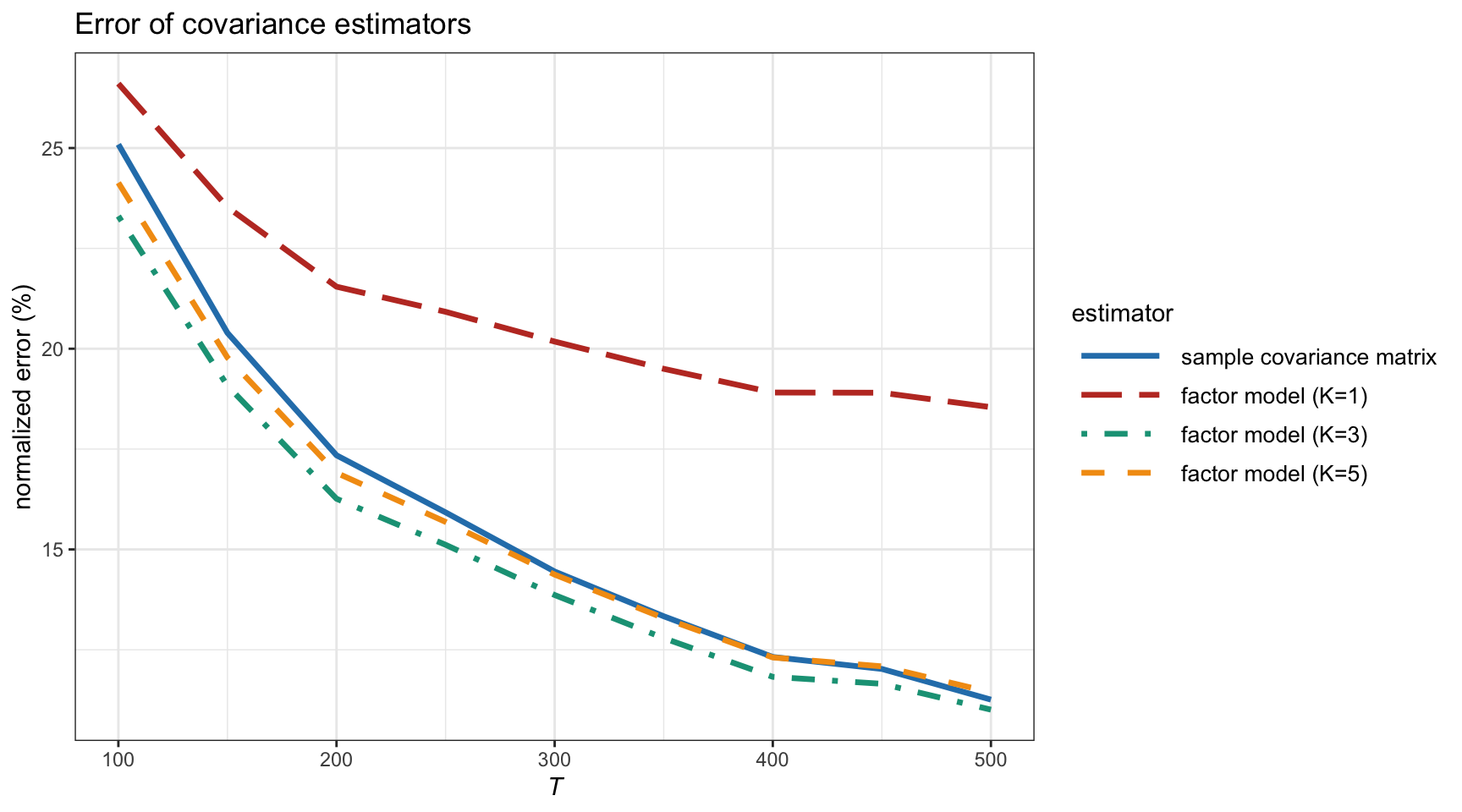
Figure 3.14: Estimation error of covariance matrix under factor modeling versus number of observations (with \(N=100\)).
3.6.3 Black-Litterman model
The Black-Litterman model was proposed in 1991 (Black and Litterman, 1991) and has become standard material in finance as described in many textbooks, such as (Fabozzi et al., 2010) and (Meucci, 2005). It is a mathematical technique to combine the parameter estimation based on the historical observation of the past \(T\) samples \(\bm{x}_1,\dots,\bm{x}_T\) with some prior information on these parameters.
The Black-Litterman model considers the following two components:
Market equilibrium: One source of information for \(\bmu\) is the market, e.g., the sample mean \(\hat{\bmu}=\frac{1}{T} \sum_{t=1}^T \bm{x}_t\). We can explicitly write this estimate \(\bm{\pi}=\hat{\bmu}\) in terms of the actual \(\bmu\) and the estimation error: \[\begin{equation} \bm{\pi} = \bmu + \bm{\epsilon}, \tag{3.17} \end{equation}\] where the error component \(\bm{\epsilon}\) is assumed zero-mean and with covariance matrix \(\tau \bSigma\). The parameter \(\tau\) can be selected via cross-validation or simply chosen as \(\tau = 1/T\) (i.e., the more observations the less uncertainty on the market equilibrium).
Investor’s views: Suppose we have \(K\) views summarized from investors written in the form \[\begin{equation} \bm{v} = \bm{P}\bmu + \bm{e}, \tag{3.18} \end{equation}\] where \(\bm{v} \in \R^K\) and \(\bm{P} \in \R^{K\times N}\) characterize the absolute or relative views and the error term \(\bm{e}\) is assumed zero-mean with covariance \(\bm{\Omega}\), which measures the uncertainty of the views. Exactly how to obtain such views is the secret of each investor.
Example 3.1 (Quantitative investor's views) Suppose there are \(N=5\) stocks and two independent views on them (Fabozzi et al., 2010):
- Stock 1 will have a return of 1.5% with standard deviation of 1%.
- Stock 3 will outperform Stock 2 by 4% with a standard deviation of 1%.
Mathematically, we can express these two views as \[ \begin{bmatrix} 1.5\%\\ 4\% \end{bmatrix} = \begin{bmatrix} 1 & 0 & 0 & 0 & 0\\ 0 & -1 & 1 & 0 & 0 \end{bmatrix} \bmu + \bm{e}, \] with the covariance of \(\bm{e}\) given by \(\bm{\Omega} = \begin{bmatrix} 1\%^2 & 0\\ 0 & 1\%^2 \end{bmatrix}\).
In some occasions, the investor may only have qualitative views (as opposed to quantitative ones), i.e., only matrix \(\bm{P}\) is specified while the views \(\bm{v}\) and the uncertainty \(\bm{\Omega}\) are undefined. Then, one can choose them as follows (Meucci, 2005): \[ v_i = \left(\bm{P}\bm{\pi}\right)_i + \eta_i\sqrt{\left(\bm{P}\bSigma\bm{P}^\T\right)_{ii}} \qquad i=1,\dots,K, \] where \(\eta_i \in \{-\beta, -\alpha, +\alpha, +\beta\}\) defines “very bearish”, “bearish”, “bullish”, and “very bullish” views, respectively (typical choices are \(\alpha=1\) and \(\beta=2\)); and, as for the uncertainty, \[ \bm{\Omega} = \frac{1}{c}\bm{P}\bSigma\bm{P}^\T, \] where the scatter structure of uncertainty is inherited from the market volatilities and correlations, and \(c \in (0,\infty)\) represents the overall level of confidence in the views.
An alternative to the previous market equilibrium \(\bm{\pi}=\hat{\bmu}\) can be derived from the CAPM model in (3.13) as \[ \bm{\pi} = \bm{\beta} \left(\E\left[f^\textm{mkt}]\right] - r_f\right). \]
Merging the market equilibrium with the views
The combination of the market equilibrium and the investor’s views can be mathematically formulated in a variety of ways, ranging from least squares formulations, through maximum likelihood, and even different Bayesian formulations. Interestingly, the solution is the same (or very similar) as we briefly overview next in three particular formulations.
Weighted least squares formulation: First, we rewrite the equations (3.17) and (3.18) in a more compact way as \[ \bm{y} = \bm{X}\bmu + \bm{n}, \] where \(\bm{y} = \begin{bmatrix} \bm{\pi}\\ \bm{v}\end{bmatrix}\), \(\bm{X} = \begin{bmatrix} \bm{I}\\ \bm{P}\end{bmatrix}\), and the covariance matrix of the noise term \(\bm{n}\) is given by \(\bm{V} = \begin{bmatrix} \tau \bSigma & \bm{0}\\ \bm{0} & \bm{\Omega}\end{bmatrix}\). Then we can formulate the problem as a weighted least squares problem (Feng and Palomar, 2016): \[ \begin{array}{ll} \underset{\bmu}{\textm{minimize}} & \left(\bm{y} - \bm{X}\bmu \right)^\T\bm{V}^{-1}\left(\bm{y} - \bm{X}\bmu \right), \end{array} \] with solution \[\begin{equation} \begin{aligned} \bmu_{\textm{BL}} &= \left(\bm{X}^\T\bm{V}^{-1}\bm{X}\right)^{-1}\bm{V}^{-1}\bm{y}\\ &= \left((\tau\bSigma)^{-1} + \bm{P}^\T\bm{\Omega}^{-1}\bm{P}\right)^{-1}\left((\tau\bSigma)^{-1}\bm{\pi} + \bm{P}^\T\bm{\Omega}^{-1}\bm{v}\right), \end{aligned} \tag{3.19} \end{equation}\] which has covariance matrix \[\begin{equation} \textm{Cov}(\bmu_{\textm{BL}}) = \left((\tau\bSigma)^{-1} + \bm{P}^\T\bm{\Omega}^{-1}\bm{P}\right)^{-1}. \tag{3.20} \end{equation}\]
Original Bayesian formulation: The original formulation in (Black and Litterman, 1991) assumes prior Gaussian distributions. In particular, the returns are modeled as \(\bm{x} \sim \mathcal{N}(\bmu,\bSigma)\), where \(\bSigma\) is assumed known but now \(\bmu\) is modeled random with a Gaussian distribution: \[ \bmu \sim \mathcal{N}(\bm{\pi},\tau\bSigma), \] where \(\bm{\pi}\) represents the best guess for \(\bmu\) and \(\tau\bSigma\) the uncertainty of this guess. Note that this implies that \(\bm{x} \sim \mathcal{N}(\bm{\pi},(1 + \tau)\bSigma)\). The views are also modeled following a Gaussian distribution: \[ \bm{P}\bmu \sim \mathcal{N}(\bm{v},\bm{\Omega}). \] Then, the posterior distribution of \(\bmu\) given \(\bm{v}\) and \(\bm{\Omega}\) follows from Bayes formula as \[ \bmu \mid \bm{v},\bm{\Omega} \sim \mathcal{N}\left(\bmu_{\textm{BL}},\bSigma_{\textm{BL}}\right), \] where the posterior mean is exactly like the previous LS solution in (3.19) and \(\bSigma_{\textm{BL}} = \textm{Cov}(\bmu_{\textm{BL}}) + \bSigma\) with \(\textm{Cov}(\bmu_{\textm{BL}})\) in (3.20). By using the matrix inversion lemma, we can further rewrite the Black-Litterman estimators for the mean and covariance matrix as \[\begin{equation} \begin{aligned} \bmu_{\textm{BL}} &= \bm{\pi} + \tau\bSigma\bm{P}^\T\left(\tau\bm{P}\bSigma\bm{P}^\T + \bm{\Omega}\right)^{-1}(\bm{v} - \bm{P}\bm{\pi})\\ \bSigma_{\textm{BL}} &= (1+\tau)\bSigma - \tau^2\bSigma\bm{P}^\T\left(\tau\bm{P}\bSigma\bm{P}^\T + \bm{\Omega}\right)^{-1}\bm{P}\bSigma. \end{aligned} \tag{3.21} \end{equation}\]
Alternative Bayesian formulation: It is worth mentioning a variation of the original Bayesian formulation in (Meucci, 2005), where the views are modeled on the random returns, \(\bm{v} = \bm{P}\bm{x} + \bm{e}\), unlike (3.18) where the views are on \(\bmu\). In this case, one can similarly derive the posterior distribution of the returns with a result similar to (3.21).
As a final observation, it is insightful to consider the two extremes:
- \(\tau = 0\): we give total accuracy to the market equilibrium and, as expected, we get \[ \bmu_{\textm{BL}} = \bm{\pi}. \]
- \(\tau \rightarrow \infty\): we give no value at all to the market equilibrium and, therefore, the investor’s views dominate \[ \bmu_{\textm{BL}} = \left(\bm{P}^\T\bm{\Omega}^{-1}\bm{P}\right)^{-1}\left(\bm{P}^\T\bm{\Omega}^{-1}\bm{v}\right). \] In the general case with \(0 < \tau < \infty\), \(\bmu_{\textm{BL}}\) is a weighted combination of these two extreme cases, which is actually related to the concept of shrinkage explored in Section 3.6.1.
References
The gross domestic product (GDP) is a monetary measure of the market value of all the final goods and services produced and sold in a specific time period by countries.↩︎