4.4 Volatility/Variance Modeling
Volatility clustering is a stylized fact of financial data that refers to the observation that large price changes tend to be followed by large price changes (ignoring the sign), whereas small price changes tend to be followed by small price changes (Fama, 1965; Mandelbrot, 1963). This phenomenon of volatility clustering, showcased in the exploratory data analysis in Section 2.4 of Chapter 2, clearly reveals temporal structure that can potentially be exploited through proper modeling.
Section 4.3 has focused on using the temporal structure for the purpose of mean modeling or modeling of the conditional expected return \(\bm{\mu}_t\) in (4.1) under a constant conditional variance. We now explore a variety of models to exploit the temporal structure in the modeling of the conditional variance \(\bm{\Sigma}_t\).
Unless otherwise stated, we will focus on the univariate case (single asset) for simplicity. Therefore, the objective is to compute the expectation of the future variance of the time series at time \(t\) based on the past observations \(\mathcal{F}_{t-1}\), that is, \(\textm{Var}[\epsilon_t \mid \mathcal{F}_{t-1}] = \E[\epsilon_t^2]\) in (4.1), where \(\epsilon_t = x_t - \mu_t\) is the forecasting error or innovation term. In practice, since the magnitude of \(\mu_t\) is much smaller than that of the observed noisy data \(x_t\), one can also focus, for simplicity and with a negligible effect in accuracy, on \(\E[x_t^2 \mid \mathcal{F}_{t-1}]\). Note that the volatility is not a directly observable quantity (although meaningful proxies can be used) and defining an error measure requires some careful thought (Poon and Granger, 2003); alternatively, a visual inspection of the result is also of practical relevance.
The topic of volatility modeling or variance modeling is standard material in many textbooks (Lütkepohl, 2007; Ruppert and Matteson, 2015; Tsay, 2010), as well as some specific overview papers (Bollerslev et al., 1992; Poon and Granger, 2003; Taylor, 1994).
4.4.1 Moving Average (MA)
Under the i.i.d. model in (3.1), the residual is distributed as \(\epsilon_t \sim \mathcal{N}(0,\sigma^2)\) and the simplest way to estimate its variance \(\sigma^2 = \E[\epsilon_t^2]\) is by taking the average of the squared values. In practice, the variance and volatility are slowly time-varying, denoted by \(\sigma_t^2\) and \(\sigma_t\), respectively. The volatility envelope precisely refers to the time-varying volatility \(\sigma_t\).
To allow for a slowly time-varying variance, we can use a moving average or rolling means (like in Section 4.3.1) on the squared residuals: \[\begin{equation} \hat{\sigma}_t^2 = \frac{1}{q}\sum_{i=1}^q \epsilon_{t-i}^2. \tag{4.11} \end{equation}\] Figure 4.6 illustrates the volatility envelope computed via MAs of different lengths.
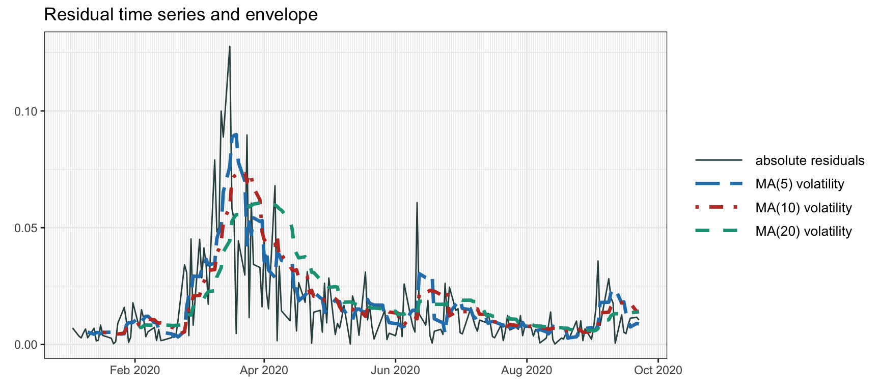
Figure 4.6: Volatility envelope with moving averages.
4.4.2 EWMA
Similarly to Section 4.3.2, we can put more weight on the recent observations. One option is to use exponential weights, which can be efficiently computed recursively as \[\begin{equation} \hat{\sigma}_t^2 = \alpha \epsilon_{t-1}^2 + (1 - \alpha) \hat{\sigma}_{t-1}^2, \tag{4.12} \end{equation}\] where \(\alpha\) (\(0\leq\alpha\leq1\)) determines the exponential decay or memory.
Figure 4.7 shows the volatility envelope computed via EWMAs of different memory. Whenever there is a large residual spike, the subsequent exponential decay of the volatility can be observed.
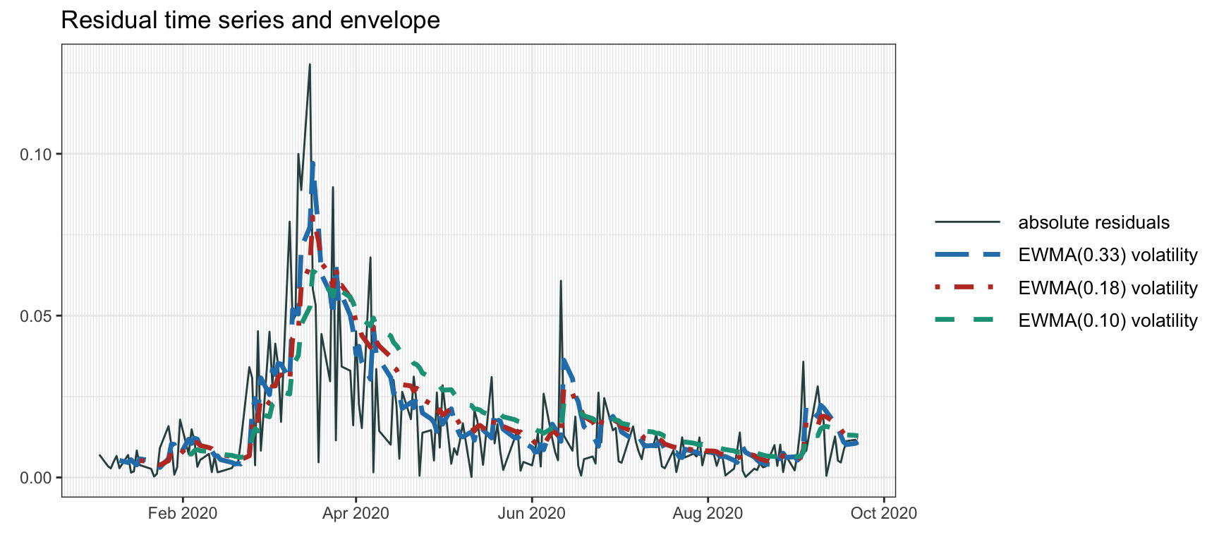
Figure 4.7: Volatility envelope with EWMA.
4.4.3 GARCH Modeling
Heteroskedasticity is the technical term that refers to the phenomenon of a time-varying variance. The autoregressive conditional heteroskedasticity (ARCH) model is one of the earliest models to deal with heteroskedasticity and, in particular, the volatility clustering effect.
The (linear) ARCH model of order \(q\), denoted by ARCH\((q)\), was proposed by Engle (1982)18 and it is defined as \[\begin{equation} \begin{aligned} \epsilon_t &= \sigma_t z_t,\\ \sigma_t^2 &= \omega + \sum_{i=1}^q \alpha_i \epsilon_{t-i}^2, \end{aligned} \tag{4.13} \end{equation}\] where \(\epsilon_t\) is the innovation to be modeled, \(z_t\) is an i.i.d. random variable with zero mean and unit variance, \(\sigma_t\) is the slowly time-varying volatility envelope (expressed as a moving average of the past squared residuals), and the parameters of the model are \(\omega > 0\) and \(\alpha_1,\dots,\alpha_q \ge 0\).
An important limitation of the ARCH model is that the high volatility is not persistent enough (unless \(q\) is chosen very large) to capture the phenomenon of volatility clustering. This can be overcome by the generalized ARCH (GARCH) model proposed by Bollerslev (1986).
The (linear) GARCH model of orders \(p\) and \(q\), denoted by GARCH\((p,q)\), is \[\begin{equation} \begin{aligned} \epsilon_t &= \sigma_t z_t,\\ \sigma_t^2 &= \omega + \sum_{i=1}^q \alpha_i \epsilon_{t-i}^2 + \sum_{j=1}^p \beta_j \sigma_{t-j}^2, \end{aligned} \tag{4.14} \end{equation}\] where now the parameters are \(\omega > 0\), \(\alpha_1,\dots,\alpha_q \ge0\), and \(\beta_1,\dots,\beta_p \ge0\) (one technical condition to guarantee stationarity is \(\sum_{i=1}^q \alpha_i + \sum_{j=1}^p \beta_j < 1\)). This is formally an ARMA model on \(\epsilon_{t}^2\). The recursive component in \(\sigma_t\) allows the volatility to be more persistent in time.
Since the ARCH and GARCH models were proposed in the 1980s, a wide range of extensions and variations, including nonlinear recursions and non-Gaussian distributed innovations, have appeared in the econometric literature, cf. Bollerslev et al. (1992), Lütkepohl (2007), Tsay (2010), and Ruppert and Matteson (2015). In the case of intraday financial data, the model is extended to include the intraday pattern, the so-called “volatility smile” (Engle and Sokalska, 2012; Xiu and Palomar, 2023).
GARCH models require the appropriate coefficients to properly fit the data and this is typically done in practice via maximum likelihood procedures. Mature and efficient software implementations are readily available in most programming languages.19
Figure 4.8 shows the volatility envelope computed via different ARCH and GARCH models. As in the EWMA case, whenever a large spike appears, a subsequent exponential decay of the volatility can be observed.
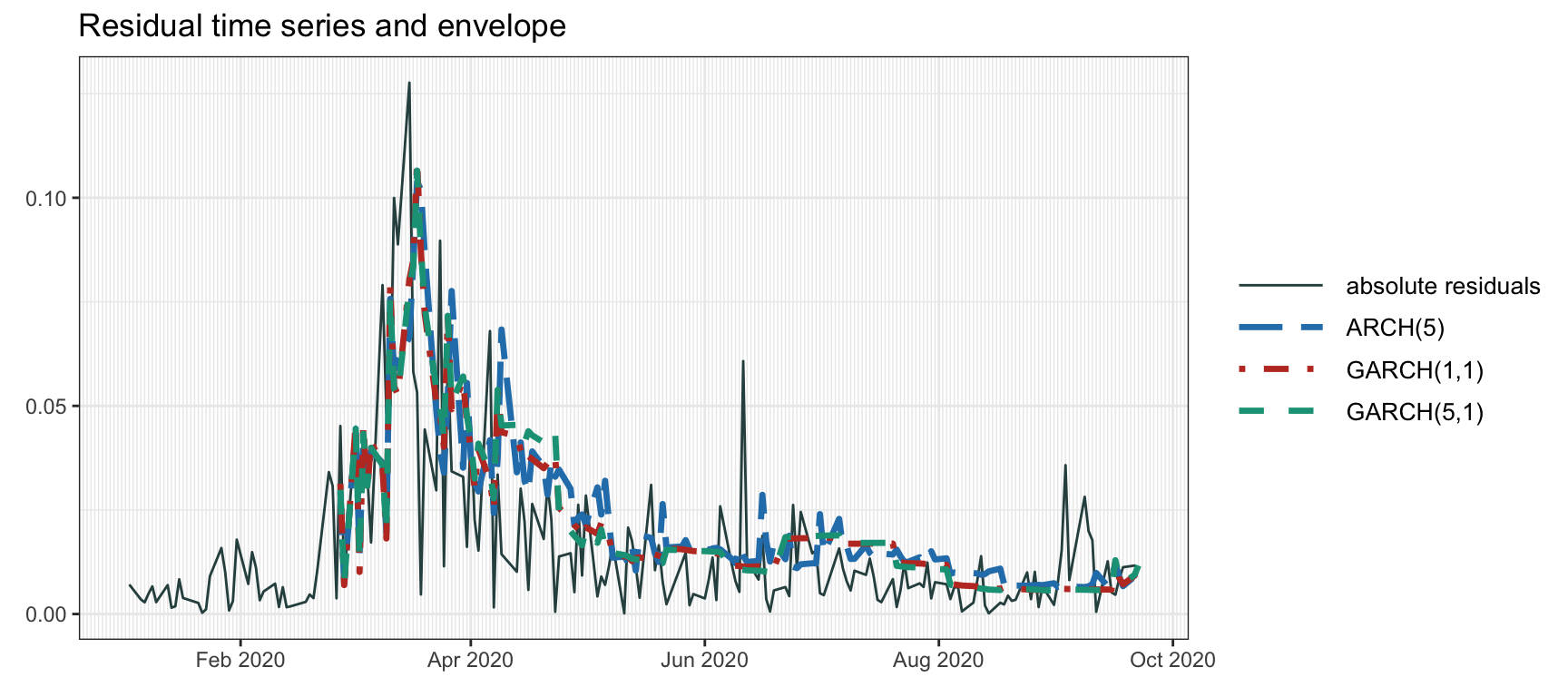
Figure 4.8: Volatility envelope with GARCH models.
Criticism of GARCH Models
GARCH models are extremely popular and well-researched in econometrics. Nevertheless, one has to admit that they are essentially “glorified” exponentially weighted moving averages. Indeed, taking the GARCH variance modeling in (4.14) and setting, for simplicity, \(p=q=1\), \(\omega=0\), and \(\beta_1 = 1 - \alpha_1\), we obtain \[ \sigma_t^2 = \alpha_1 \epsilon_{t-1}^2 + (1 - \alpha_1) \sigma_{t-1}^2, \] which looks exactly like the EWMA in (4.12). In words, GARCH models attempt to represent the volatility as a series of (unpredictable) spikes that decay exponentially over time. As a consequence, the volatility curve looks rugged and composed of overlapping exponential curves. Arguably this is not how a slowly time-varying envelope is expected to look, but nevertheless these models have enjoyed an unparalleled popularity.
In addition, the estimation of the GARCH parameters (model fitting) is extremely “data hungry.” That is, unless the number of observations is really large, estimation of the parameters becomes unreliable as illustrated with the following numerical example.20 Figure 4.9 shows a scatter plot with 1000 Monte Carlo random simulations of the parameter estimation values of a GARCH(1,1) model with \(\omega=0\), \(\alpha_1 = 0.07\), and \(\beta_1 = 0.925\) based on \(T=1000\) observations. The variation in the estimated parameters is around \(0.1\), which is quite large even though 1000 observations were used (4 years of daily data).
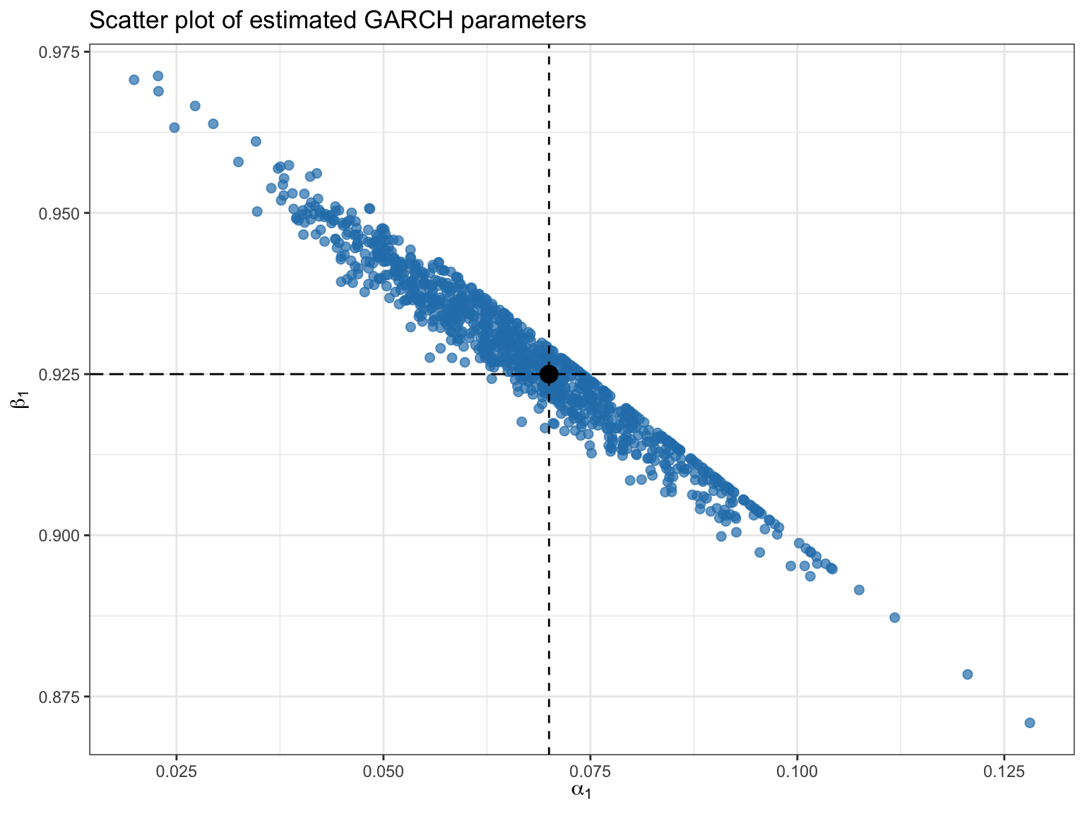
Figure 4.9: Instability in GARCH model fitting.
4.4.4 Stochastic Volatility Modeling
In 1982, Taylor proposed in a seminal work to model the volatility probabilistically via a state-space model termed the stochastic volatility (SV) model (Taylor, 1982). Even though SV and GARCH were proposed in the same year, SV modeling has not enjoyed the same popularity as GARCH modeling in econometrics. One possible reason is that the fitting process is theoretically more involved and computationally demanding; in fact, a maximum likelihood optimization cannot be exactly formulated for SV (Kim et al., 1998; Poon and Granger, 2003). Nevertheless, as explored in later in Section 4.4.5, Kalman filtering can be efficiently used as a good practical approximation (A. Harvey et al., 1994; Ruiz, 1994).
The SV model is conveniently written in terms of the log-variance, \(h_t = \textm{log}(\sigma_t^2)\), as \[\begin{equation} \begin{aligned} \epsilon_t &= \textm{exp}(h_t/2) z_t,\\ h_t &= \gamma + \phi h_{t-1} + \eta_t, \end{aligned} \tag{4.15} \end{equation}\] where the first equation is equivalent to that in the ARCH and GARCH models, \(\epsilon_t = \sigma_t z_t\), and the second equation models the volatility dynamics with parameters \(\gamma\) and \(\phi\) in a stochastic way via the residual term \(\eta_t\).
To gain more insight, we can rewrite the volatility state transition equation from (4.15) in terms of \(\sigma_t^2\) as \[ \textm{log}(\sigma_t^2) = \gamma + \phi \, \textm{log}(\sigma_{t-1}^2) + \eta_t, \] which allows a clearer comparison with a GARCH(1,1) model: \[ \sigma_t^2 = \omega + \beta_1 \sigma_{t-1}^2 + \alpha_1 \epsilon_{t-1}^2. \] As we can observe, the main difference (apart from modeling the log variance instead of the variance, which has also been done in the exponential GARCH model) appears in the noise term \(\eta_t\) in the volatility state transition equation. This difference may seem tiny and insignificant, but it actually makes it fundamentally different to GARCH models where the time-varying volatility is assumed to follow a deterministic instead of stochastic evolution.
SV models, albeit not having received the same attention as GARCH models, are still covered in some excellent overview papers (A. Harvey et al., 1994; Kim et al., 1998; Poon and Granger, 2003; Ruiz, 1994; Taylor, 1994) and standard textbooks (Tsay, 2010).
SV modeling requires the appropriate coefficients to properly fit the data. Unlike GARCH models, this coefficient estimation process is mathematically more involved and computationally more demanding. Typically, computationally intensive Markov chain Monte Carlo (MCMC) algorithms are employed (Kim et al., 1998).21 In the next section, we consider an efficient quasi-likelihood method via Kalman filtering (A. Harvey et al., 1994; Ruiz, 1994).
Figure 4.10 displays the volatility envelope calculated using the SV model. As can be observed, the envelope appears smooth, contrasting with the rugged overlap of decaying exponential curves observed in GARCH modeling.
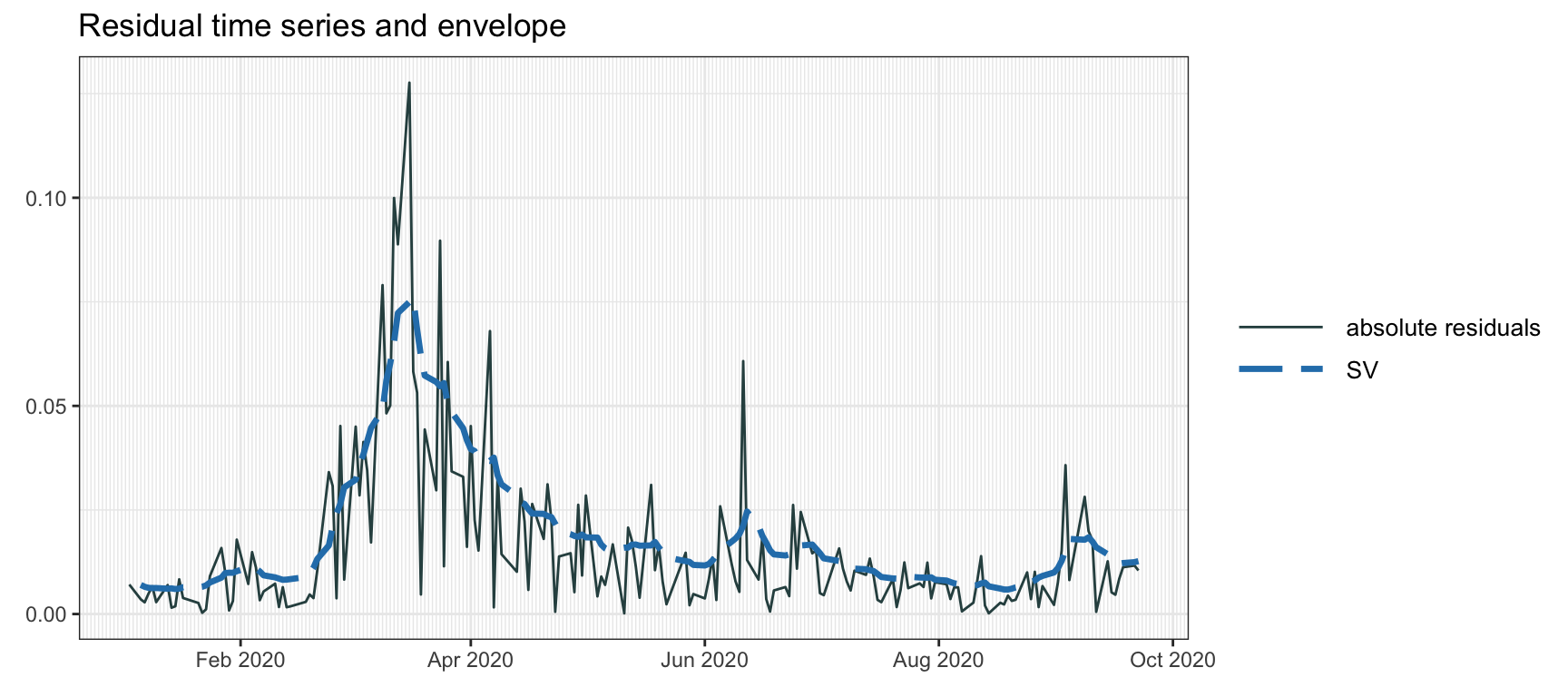
Figure 4.10: Volatility envelope with SV modeling via MCMC.
4.4.5 Kalman Modeling
The SV model can be written with a state-space representation and approximately solved via the Kalman filtering as described next (A. Harvey et al., 1994; Ruiz, 1994; Zivot et al., 2004).
Taking the logarithm in the SV squared observation equation in (4.15), \(\epsilon_t^2 = \textm{exp}(h_t) z_t^2\), gives \[ \textm{log}(\epsilon_t^2) = h_t + \textm{log}(z_t^2), \] where \(\textm{log}(z_t^2)\) is a non-Gaussian i.i.d. process. If a Gaussian distribution \(z_t \sim \mathcal{N}(0, 1)\) is assumed, then the mean and variance of \(\textm{log}(z_t^2)\) are \(\psi(1/2) - \textm{log}(1/2) \approx -1.27\) and \(\pi^2/2\), respectively, where \(\psi(\cdot)\) denotes the digamma function. Similarly, if a heavy-tailed \(t\) distribution is assumed with \(\nu\) degrees of freedom, then the mean is approximately \(-1.27 - \psi(\nu/2) + \textm{log}(\nu/2)\) and the variance \(\pi^2/2 + \psi'(\nu/2)\), where \(\psi'(\cdot)\) is the trigamma function.
Thus, under the Gaussian assumption for \(z_t\), the SV model in (4.15) can be approximated as \[\begin{equation} \begin{aligned} \textm{log}(\epsilon_t^2) &= -1.27 + h_t + \xi_t,\\ h_t &= \gamma + \phi h_{t-1} + \eta_t, \end{aligned} \tag{4.16} \end{equation}\] where \(\xi_t\) is a non-Gaussian i.i.d. process with zero mean and variance \(\pi^2/2\), and the parameters of the model are \(\gamma\), \(\phi\), and the variance \(\sigma_{\eta}^2\) of \(\eta_t\). This model fits the state-space representation in (4.2); however, since \(\xi_t\) is not Gaussian then Kalman filtering will not produce optimal results.
One particular case of (4.16) is the random walk plus noise model with \(\gamma=0\) and \(\phi = 1\): \[\begin{equation} \begin{aligned} \textm{log}(\epsilon_t^2) &= -1.27 + h_t + \xi_t,\\ h_t &= h_{t-1} + \eta_t, \end{aligned} \tag{4.17} \end{equation}\] with the single remaining parameter \(\sigma_{\eta}^2\).
It is important to realize that the different choices of model will produce different volatility envelopes. Since the volatility is unobservable, it is not clear how to choose the best model. In some cases, however, it is possible to observe the volatility, called “realized volatility,” and then the model can be fitted in a better way. One example is when higher-frequency data is available and can be used to compute the realized volatility during the slower-frequency period, for example, hourly data can be used to estimate the daily volatility.
Figure 4.11 shows the volatility envelope forecast according to the SV model via Kalman filtering. If a noncausal envelope is allowed, then we can instead use Kalman smoothing as in Figure 4.12, which clearly produces much smoother and more accurate envelopes at the expense of using noncausal data.
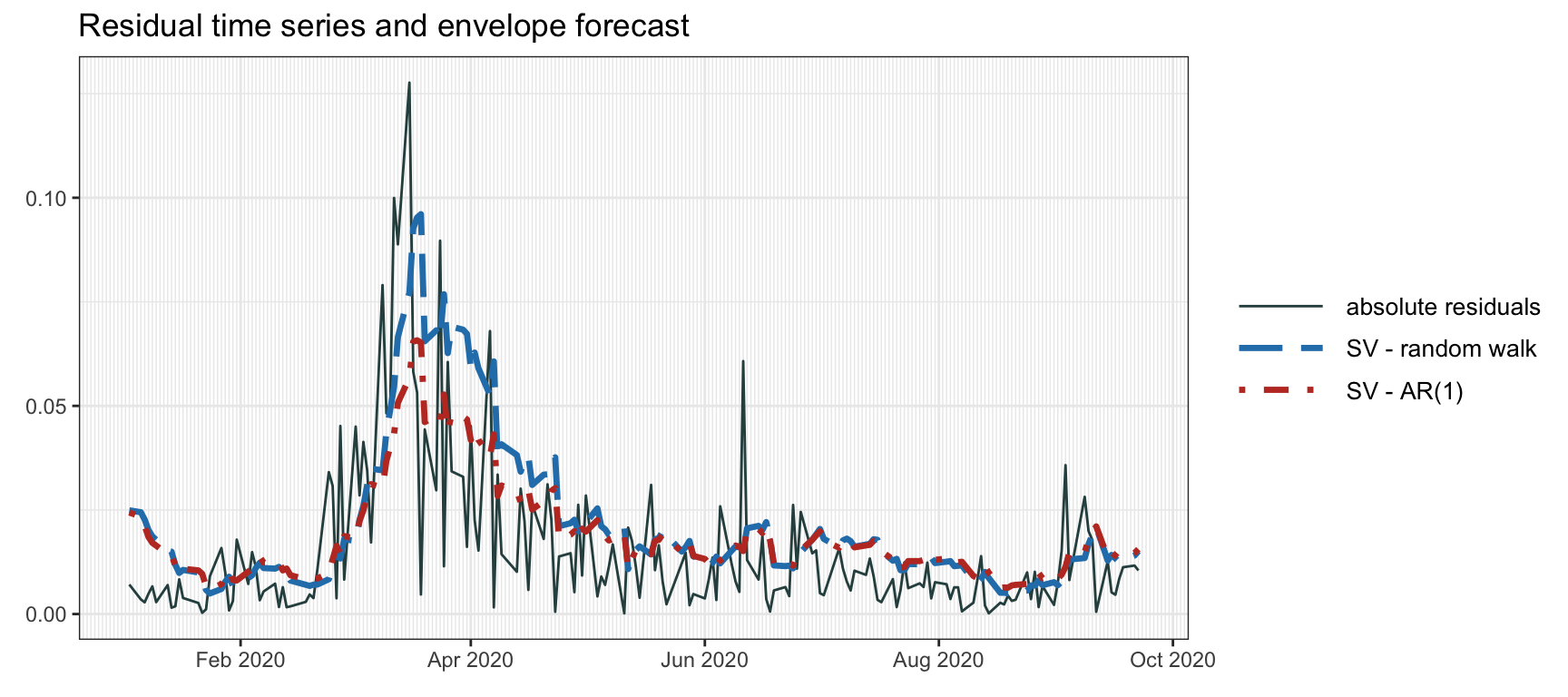
Figure 4.11: Volatility envelope with SV modeling via Kalman filter.
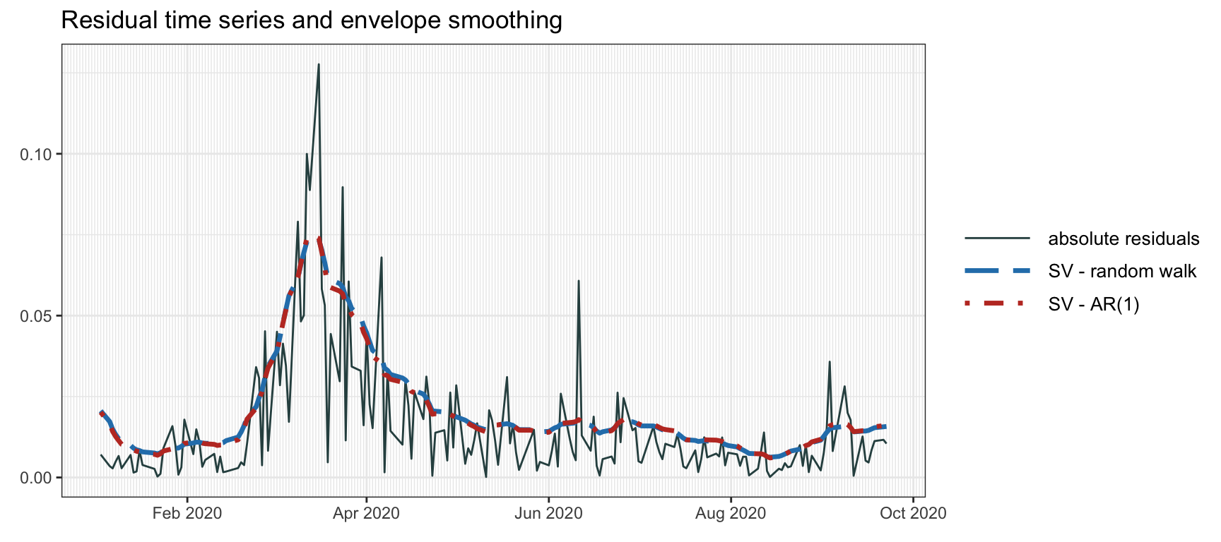
Figure 4.12: Volatility envelope with SV modeling via Kalman smoother.
4.4.6 Extension to the Multivariate Case
All the previous (univariate) volatility models can be applied to \(N\) assets on an asset-by-asset basis. Nevertheless, it may be advantageous to use a multivariate model that can better model the common volatility clustering observed in market data.
Multivariate EWMA
To start with, following the univariate EMWA volatility modeling from Section 4.4.2, we can easily extend the univariate estimation in (4.12) to the multivariate case as \[ \hat{\bm{\Sigma}}_t = \alpha \bm{\epsilon}_{t-1}\bm{\epsilon}_{t-1}^\T + (1 - \alpha) \hat{\bm{\Sigma}}_{t-1}, \] where \(\bm{\epsilon}_t = \bm{x}_t - \bmu_t \in \R^N\) is the forecasting error vector and \(\alpha\) is the smoothing parameter that determines the exponential decay or memory. This model can easily be extended so that each asset has a different smoothing parameter (Tsay, 2013).
Multivariate GARCH
Numerous attempts have been made to extend the univariate GARCH models (see Section 4.4.3) to the multivariate case (Bollerslev et al., 1992; Lütkepohl, 2007; Tsay, 2013). Similarly to the univariate cases in (4.13) and (4.14), the forecasting error vector can be conveniently decomposed as \[ \bm{\epsilon}_t = \bm{\Sigma}_t^{1/2} \bm{z}_t, \] where \(\bm{z}_t \in \R^{N}\) is a zero-mean random vector with identity covariance matrix and the volatility is modeled by the matrix \(\bm{\Sigma}_t^{1/2} \in \R^{N\times N}\), which is the square-root matrix of \(\bm{\Sigma}_t\) (satisfying \(\bm{\Sigma}_t^{\T/2} \bm{\Sigma}_t^{1/2} = \bm{\Sigma}_t\)). In other words, \(\bm{\Sigma}_t\) is the covariance matrix that generalizes the variance \(\sigma_t^2\) in the univariate case and \(\bm{\Sigma}_t^{1/2}\) is the matrix generalization of the volatility \(\sigma_t\).
The complication arises when modeling the dynamics of the volatility matrix \(\bm{\Sigma}_t^{1/2}\), particularly due to the significant increase in the number of parameters when transitioning from univariate to multivariate analysis. As always, the problem with a large number of parameters is that the model will inevitably suffer from overfitting in a practical setting. A wide range of models have been proposed in the literature trying to cope with this issue; see the overview in Bollerslev et al. (1992). A naive extension is the multivariate GARCH model, which simply follows from the univariate GARCH model by vectorizing all the matrix terms (each of dimension \(N^2\)) resulting in model coefficients in the form of huge matrices of dimension \(N^2 \times N^2\). Subsequent proposals attempted to reduce the number of parameters by incorporating some structure in the matrix coefficients, such as enforcing diagonal matrices. However, the number of parameters remains on the order of \(N^2\), which is still too large to prevent overfitting.
The constant conditional correlation (CCC) model addresses the dimensionality issue by modeling the heteroskedasticity in each asset with univariate models (asset by asset) combined with a constant correlation matrix for all the assets (Bollerslev, 1990). Mathematically, the model is \[ \bm{\Sigma}_t = \bm{D}_t\bm{C}\bm{D}_t, \] where \(\bm{D}_t = \textm{Diag}(\sigma_{1,t},\dots,\sigma_{N,t})\) represents the time-varying conditional volatilities of each of the assets and the matrix \(\bm{C}\) is the constant correlation matrix. This model is very convenient in practice because it avoids the explosion of the number of parameters. Basically, the volatility envelope of each asset is first modeled individually and removed from the data as \(\bar{\bm{\epsilon}}_t = \bm{D}_t^{-1}\bm{\epsilon}_t\), and then the correlation structure of the multivariate data \(\bar{\bm{\epsilon}}_t\) (with approximately constant volatility) is obtained. A disadvantage of this model is the fact that the correlation structure is fixed.
The dynamic conditional correlation (DCC) model precisely addresses the drawback of the CCC model and allows the correlation matrix to change over time, but using a single scalar parameter to avoid overfitting (Engle, 2002). To be precise, the time-varying correlation matrix \(\bm{C}_t\) is obtained via an exponentially weighted moving average of the data with removed volatility \(\bar{\bm{\epsilon}}_t\), \[ \bm{Q}_t = \alpha \bar{\bm{\epsilon}}_{t-1}\bar{\bm{\epsilon}}_{t-1}^\T + (1 - \alpha) \bm{Q}_{t-1}, \] with an additional normalization step in case a correlation matrix is desired (with diagonal elements equal to one): \[ \bm{C}_t = \textm{Diag}(\bm{Q}_t)^{-1/2} \bm{Q}_t \textm{Diag}(\bm{Q}_t)^{-1/2}. \] One disadvantage of this model is that it forces all the correlation coefficients to have the same memory via the same \(\alpha\), which could be further relaxed at the expense of more parameters.
Thus, the recommended procedure for building DCC models is (Tsay, 2013):
Use any of the mean modeling techniques from Section 4.3 to obtain a forecast \(\bmu_t\) and then compute the residual or error vector of the forecast \(\bm{\epsilon}_t = \bm{x}_t - \bmu_t\).
Apply any of the univariate volatility models from Section 4.4 to obtain the volatility envelopes for the \(N\) assets \((\sigma_{1,t},\dots,\sigma_{N,t})\).
Standardize each of the series with the volatility envelope, \(\bar{\bm{\epsilon}}_t = \bm{D}_t^{-1}\bm{\epsilon}_t\), so that a series with approximately constant envelope is obtained.
Compute either a fixed covariance matrix of the multivariate series \(\bar{\bm{\epsilon}}_t\) or an exponentially weighted moving average version.
It is worth mentioning that copulas are another popular approach for multivariate modeling that can be combined with DCC models (Ruppert and Matteson, 2015; Tsay, 2013).
Multivariate SV
The multivariate extension of the SV observation equation \(\epsilon_t = \textm{exp}(h_t/2) z_t\) in (4.15) is \[ \bm{\epsilon}_t = \textm{Diag}\left(\textm{exp}(\bm{h}_t/2)\right) \bm{z}_t, \] where now \(\bm{h}_t = \textm{log}(\bm{\sigma}_t^2)\) denotes the log-variance vector and \(\bm{z}_t\) is a random vector with zero mean and fixed covariance matrix \(\bm{\Sigma}_z\). The covariance matrix modeled in this way can be expressed as \(\bSigma_t = \textm{Diag}\left(\textm{exp}(\bm{h}_t/2)\right) \bm{\Sigma}_z \textm{Diag}\left(\textm{exp}(\bm{h}_t/2)\right)\), which has the same form as the CCC model, that is, the covariance matrix can be decomposed into the time-varying volatilities and the fixed matrix that models the fixed correlations.
Similarly to (4.16), taking the logarithm of the observation equation leads to the following approximated state-space model (A. Harvey et al., 1994): \[\begin{equation} \begin{aligned} \textm{log}\left(\bm{\epsilon}_t^2\right) &= -1.27\times\bm{1} + \bm{h}_t + \bm{\xi}_t,\\ \bm{h}_t &= \bm{\gamma} + \textm{Diag}\left(\bm{\phi}\right) \bm{h}_{t-1} + \bm{\eta}_t, \end{aligned} \tag{4.18} \end{equation}\] where now \(\bm{\xi}_t\) is a non-Gaussian i.i.d. vector process with zero mean and a covariance matrix \(\bm{\Sigma}_{\xi}\) that can be obtained from \(\bm{\Sigma}_z\) (A. Harvey et al., 1994). In particular, if \(\bm{\Sigma}_z = \bm{I}\) then \(\bm{\Sigma}_{\xi} = \pi^2/2 \times \bm{I}\), which then reduces to an asset-by-asset model.
Similarly, the multivariate version of the random walk plus noise model in (4.17) is \[\begin{equation} \begin{aligned} \textm{log}\left(\bm{\epsilon}_t^2\right) &= -1.27\times\bm{1} + \bm{h}_t + \bm{\xi}_t\\ \bm{h}_t &= \bm{h}_{t-1} + \bm{\eta}_t. \end{aligned} \tag{4.19} \end{equation}\]
Other extensions of SV, including common factors and heavy-tailed distributions, have also been considered (A. Harvey et al., 1994).
References
Robert F. Engle was awarded the 2003 Sveriges Riksbank Prize in Economic Sciences in Memory of Alfred Nobel “for methods of analyzing economic time series with time-varying volatility (ARCH).” ↩︎
The R packages
rugarchandfGarchimplement algorithms for fitting a wide range of different GARCH models to time series data (Ghalanos, 2022; Wuertz et al., 2022). ↩︎Patrick Burns delivered an insightful presentation at the Imperial College Algorithmic Trading Conference on 8 December, 2012, exposing the limitations of GARCH models in favor of stochastic volatility models.↩︎
The R package
stochvolimplements an MCMC algorithm for fitting SV models (Kastner, 2016). The Python packagePyMCcontains a MCMC methods that can be used for SV modeling. ↩︎