15.6 Kalman Filtering for Pairs Trading
A key component in pairs trading is the construction of a mean-reverting spread \[ z_{t} = y_{1t} - \gamma \, y_{2t} = \mu + r_t, \] where \(\gamma\) is the hedge ratio, \(\mu\) is the mean, and \(r_t\) is the zero-mean residual. Then the trading strategy will properly size the trade depending on the distance of the spread \(z_{t}\) from the equilibrium value \(\mu\).
Construction of the spread requires careful estimation of the hedge ratio \(\gamma\), as well as the mean of the spread \(\mu\). The traditional way is to employ least squares regression. In practice, the hedge ratio and the mean will slowly change over time and then the least squares solution should be recomputed on a rolling-window basis. However, it is better to employ a more sophisticated time-varying modeling and estimation technique based on state-space modeling and the Kalman filter (Chan, 2013; Feng and Palomar, 2016).
15.6.1 Spread Modeling via Least Squares
The method of least squares (LS) dates back to 1795 when Gauss used it to study planetary motions. It deals with the linear model \(\bm{y} = \bm{A}\bm{x} + \bm{\epsilon}\) by solving the problem (Kay, 1993; Scharf, 1991) \[ \begin{array}{ll} \underset{\bm{x}}{\textm{minimize}} & \left\Vert \bm{y} - \bm{A}\bm{x} \right\Vert_2^2, \end{array} \] whose solution gives the least squares estimate \(\hat{\bm{x}}=\left(\bm{A}^\T\bm{A}\right)^{-1}\bm{A}^\T\bm{y}\). In addition, the covariance matrix of the estimate \(\hat{\bm{x}}\) is given by \(\sigma_\epsilon^2\left(\bm{A}^\T\bm{A}\right)^{-1}\), where \(\sigma_\epsilon^2\) is the variance of the residual \(\bm{\epsilon}\) (in practice, the variance of the estimated residual \(\hat{\bm{\epsilon}} = \bm{y} - \bm{A}\hat{\bm{x}}\) can be used instead).
In our context of spread modeling, we want to fit \(y_{1t} \approx \mu + \gamma \, y_{2t}\) based on \(T\) observations, so the LS formulation becomes \[ \begin{array}{ll} \underset{\mu,\gamma}{\textm{minimize}} & \left\Vert \bm{y}_1 - \left(\mu \bm{1} + \gamma \, \bm{y}_2\right) \right\Vert_2^2, \end{array} \] where the vectors \(\bm{y}_1\) and \(\bm{y}_2\) contain the \(T\) observations of the two time series, and \(\bm{1}\) is the all-ones vector. The solution gives the estimates \[ \begin{bmatrix} \begin{array}{ll} \hat{\mu} \\ \hat{\gamma} \end{array} \end{bmatrix} = \begin{bmatrix} \begin{array}{ll} \bm{1}^\T\bm{1} & \bm{1}^\T\bm{y}_2\\ \bm{y}_2^\T\bm{1} & \bm{y}_2^\T\bm{y}_2 \end{array} \end{bmatrix}^{-1} \begin{bmatrix} \begin{array}{ll} \bm{1}^\T\bm{y}_1\\ \bm{y}_2^\T\bm{y}_1 \end{array} \end{bmatrix}. \]
In practice, it is more convenient to first remove the mean of \(\bm{y}_1\) and \(\bm{y}_2\) to produce the centered versions \(\bar{\bm{y}}_1\) and \(\bar{\bm{y}}_2\), then estimate the hedge ratio as \[ \hat{\gamma} = \frac{\bar{\bm{y}}_2^\T \bar{\bm{y}}_1}{\bar{\bm{y}}_2^\T \bar{\bm{y}}_2}, \] and finally compute the sample mean of \(\bm{y}_1 - \hat{\gamma} \, \bm{y}_2\): \[ \hat{\mu} = \frac{\bm{1}^\T(\bm{y}_1 - \hat{\gamma} \, \bm{y}_2)}{T}. \]
The variance of these estimates is given by \[ \begin{array}{ll} \textm{Var}[\hat{\gamma}] &= \frac{1}{T} \; \sigma_\epsilon^2 / \sigma_2^2,\\ \textm{Var}[\hat{\mu}] &= \frac{1}{T} \;\sigma_\epsilon^2, \end{array} \] where \(\sigma_2^2\) is the variance of \(\bm{y}_2\) and \(\sigma_\epsilon^2\) is the variance of the residual \(\bm{\epsilon}\).
It is important to reiterate that in practice the hedge ratio and the mean will slowly change over time, as denoted by \(\gamma_t\) and \(\mu_t\), and the least squares solution must be recomputed on a rolling-window basis (based on a lookback window of past samples). Nevertheless, this time-varying case is better handled with Kalman filtering, as described next.
15.6.2 Primer on the Kalman Filter
State-space modeling provides a unified framework for treating a wide range of problems in time series analysis. It can be thought of as a universal and flexible modeling approach with a very efficient algorithm, the Kalman filter. The basic idea is to assume that the evolution of the system over time is driven by a series of unobserved or hidden values, which can only be measured indirectly through observations of the system output. This model can be used for filtering, smoothing, and forecasting. Here we provide a concise summary; more details on state-space modeling and Kalman filtering can be found in Section 4.2 of Chapter 4.
The Kalman filter, which was employed by NASA during the 1960s in the Apollo program, now boasts a vast array of technological applications. It is commonly utilized in the guidance, navigation, and control of vehicles, including aircraft, spacecraft, and maritime vessels. It has also found applications in time series analysis, signal processing, and econometrics. More recently, it has become a key component in robotic motion planning and control, as well as trajectory optimization.
State-space models and Kalman filtering are mature topics with excellent textbooks available such as the classical references B. D. O. Anderson and Moore (1979) and Durbin and Koopman (2012), which was originally published in 2001. Other textbook references on time series and the Kalman filter include Brockwell and Davis (2002), Shumway and Stoffer (2017), A. Harvey (1989) and, in particular, for financial time series, Zivot et al. (2004), Tsay (2010), Lütkepohl (2007), and A. Harvey and Koopman (2009).
Mathematically, the Kalman filter is based on the following linear Gaussian state-space model with discrete time \(t=1,\dots,T\) (Durbin and Koopman, 2012): \[ \qquad\qquad \begin{aligned} \bm{y}_t &= \bm{Z}_t\bm{\alpha}_t + \bm{\epsilon}_t\\ \bm{\alpha}_{t+1} &= \bm{T}_t\bm{\alpha}_t + \bm{\eta}_t \end{aligned} \quad \begin{aligned} & \textm{(observation equation)},\\ & \textm{(state equation)}, \end{aligned} \] where \(\bm{y}_t\) denotes the observations over time with observation matrix \(\bm{Z}_t\), \(\bm{\alpha}_t\) represents the unobserved or hidden internal state with state transition matrix \(\bm{T}_t\), and the two noise terms \(\bm{\epsilon}_t\) and \(\bm{\eta}_t\) are Gaussian distributed with zero mean and covariance matrices \(\bm{H}\) and \(\bm{Q}\), respectively, that is, \(\bm{\epsilon}_t \sim \mathcal{N}(\bm{0},\bm{H})\) and \(\bm{\eta}_t \sim \mathcal{N}(\bm{0},\bm{Q})\). The initial state can be modeled as \(\bm{\alpha}_1 \sim \mathcal{N}(\bm{a}_1,\bm{P}_1)\). Mature and efficient software implementations are readily available (Helske, 2017; Holmes et al., 2012; Petris and Petrone, 2011; Tusell, 2011).66
The parameters of the state-space model (i.e., \(\bm{Z}_t\), \(\bm{T}_t\), \(\bm{H}\), \(\bm{Q}\), \(\bm{a}_1\), and \(\bm{P}_1\)) can be either provided by the user (if known) or inferred from the data with algorithms based on the maximum likelihood method. Again, mature and efficient software implementations are available for this parameter fitting (Holmes et al., 2012).67
To be more precise, the Kalman filter is a very efficient algorithm to optimally characterize the distribution of the hidden state at time \(t\), \(\bm{\alpha}_t\), in a causal manner. In particular, \(\bm{\alpha}_{t|t-1}\) and \(\bm{\alpha}_{t|t}\) denote the expected value given the observations up to time \(t-1\) and \(t\), respectively. These quantities can be efficiently computed using a “forward pass” algorithm that goes from \(t=1\) to \(t=T\) in a recursive way, so that it can operate in real time (Durbin and Koopman, 2012).
15.6.3 Spread Modeling via Kalman
In our context of spread modeling, we want to model \(y_{1t} \approx \mu_t + \gamma_t \, y_{2t}\), where now \(\mu_t\) and \(\gamma_t\) change slowly over time. This can be done conveniently via a state-space modeling by identifying the hidden state as \(\bm{\alpha}_t = \left(\mu_t, \gamma_t\right)\), leading to \[\begin{equation} \begin{aligned} y_{1t} &= \begin{bmatrix} 1 & y_{2t} \end{bmatrix} \begin{bmatrix} \mu_t\\ \gamma_t \end{bmatrix} + \epsilon_t,\\ \begin{bmatrix} \mu_{t+1}\\ \gamma_{t+1} \end{bmatrix} &= \begin{bmatrix} 1 & 0\\ 0 & 1 \end{bmatrix} \begin{bmatrix} \mu_t\\ \gamma_t \end{bmatrix} + \begin{bmatrix} \eta_{1t}\\ \eta_{2t} \end{bmatrix} , \end{aligned} \tag{15.3} \end{equation}\] where all the noise components are independent and distributed as \(\epsilon_t \sim \mathcal{N}(0,\sigma_\epsilon^2)\), \(\eta_{1t} \sim \mathcal{N}(0,\sigma_{\mu}^2)\), and \(\eta_{2t} \sim \mathcal{N}(0,\sigma_{\gamma}^2)\), the state transition matrix is the identity \(\bm{T}=\bm{I}\), the observation matrix is \(\bm{Z}_t=\begin{bmatrix} 1 & y_{2t} \end{bmatrix}\), and the initial states are \(\mu_{1} \sim \mathcal{N}\left(\bar{\mu},\sigma_{\mu,1}^2\right)\) and \(\gamma_{1} \sim \mathcal{N}\left(\bar{\gamma},\sigma_{\gamma,1}^2\right)\).
The normalized spread, with leverage one (see (15.2)), can then be obtained as \[ z_{t} = \frac{1}{1 + \gamma_{t|t-1}} \left(y_{1t} - \gamma_{t|t-1} \, y_{2t} - \mu_{t|t-1}\right), \] where \(\mu_{t|t-1}\) and \(\gamma_{t|t-1}\) are the hidden states estimated by the Kalman algorithm.
The model parameters \(\sigma_\epsilon^2\), \(\sigma_\mu^2\), and \(\sigma_\gamma^2\) (and the initial states) can be determined by simple heuristics or optimally estimated from the data (more computationally demanding). For example, one can use initial training data of \(T^\textm{LS}\) samples to estimate \(\mu\) and \(\gamma\) via least squares, \(\mu^\textm{LS}\) and \(\gamma^\textm{LS}\), obtaining the estimated residual \(\epsilon_t^\textm{LS}\). Then the following provide an effective heuristic for the state-space model parameters: \[ \begin{aligned} \sigma_\epsilon^2 &= \textm{Var}\left[\epsilon_t^\textm{LS}\right],\\ \mu_1 &\sim \mathcal{N}\left(\mu^\textm{LS}, \frac{1}{T^\textm{LS}}\textm{Var}\left[\epsilon_t^\textm{LS}\right]\right),\\ \gamma_1 &\sim \mathcal{N}\left(\gamma^\textm{LS}, \frac{1}{T^\textm{LS}}\frac{\textm{Var}\left[\epsilon_t^\textm{LS}\right]}{\textm{Var}\left[y_{2t}\right]}\right),\\ \sigma_\mu^2 &= \alpha \times \textm{Var}\left[\epsilon_t^\textm{LS}\right],\\ \sigma_\gamma^2 &= \alpha \times \frac{\textm{Var}\left[\epsilon_t^\textm{LS}\right]}{\textm{Var}\left[y_{2t}\right]}, \end{aligned} \] where the hyper-parameter \(\alpha\) determines the ratio of the variability of the slowly time-varying hidden states to the variability of the spread.
The state-space model of the spread in (15.3) can be extended in different ways to potentially improve the performance. One simple extension involves modeling not only the hedge ratio but also its momentum or velocity. This can be done by expanding the hidden state to \(\bm{\alpha}_t = \left(\mu_t, \gamma_t, \dot{\gamma}_t\right)\), which leads to the state-space model \[\begin{equation} \begin{aligned} y_{1t} &= \begin{bmatrix} 1 & y_{2t} & 0 \end{bmatrix} \begin{bmatrix} \mu_t\\ \gamma_t\\ \dot{\gamma}_t \end{bmatrix} + \epsilon_t,\\ \begin{bmatrix} \mu_{t+1}\\ \gamma_{t+1}\\ \dot{\gamma}_{t+1} \end{bmatrix} &= \begin{bmatrix} 1 & 0 & 0\\ 0 & 1 & 1\\0 & 0 & 1 \end{bmatrix} \begin{bmatrix} \mu_t\\ \gamma_t\\ \dot{\gamma}_t \end{bmatrix} + \bm{\eta}_{t}. \end{aligned} \tag{15.4} \end{equation}\] This model makes \(\gamma_{t}\) less noisy and provides a better spread, as shown later in the numerical experiments.
Another extension of the state-space modeling in (15.3) under the concept of partial cointegration is to model the spread with an autoregressive component (Clegg and Krauss, 2018). This can be done by defining the hidden state as \(\bm{\alpha}_t = \left(\mu_t, \gamma_t, \epsilon_t\right)\), leading to \[\begin{equation} \begin{aligned} y_{1t} &= \begin{bmatrix} 1 & y_{2t} & 1 \end{bmatrix} \begin{bmatrix} \mu_t\\ \gamma_t\\ \epsilon_t \end{bmatrix},\\ \begin{bmatrix} \mu_{t+1}\\ \gamma_{t+1}\\ \epsilon_{t+1} \end{bmatrix} &= \begin{bmatrix} 1 & 0 & 0\\ 0 & 1 & 0\\0 & 0 & \rho \end{bmatrix} \begin{bmatrix} \mu_t\\ \gamma_t\\ \epsilon_t \end{bmatrix} + \bm{\eta}_{t}, \end{aligned} \tag{15.5} \end{equation}\] where \(\rho\) is a parameter to be estimated satisfying \(|\rho|<1\) (or fixed to some reasonable value like \(\rho=0.9)\).
15.6.4 Numerical Experiments
We now repeat the pairs trading experiments with market data during 2013–2022 as in Section 15.5. As before, the \(z\)-score is computed on a rolling-window basis with a lookback period of six months and pairs trading is implemented via the thresholded strategy with a threshold of \(s_0=1\). The difference is that we now employ three different methods to track the hedge ratio over time: (i) rolling least squares with lookback period of two years, (ii) basic Kalman based on (15.3) with \(\alpha=10^{-5}\), and (iii) Kalman with momentum based on (15.4) with \(\alpha=10^{-6}\). All these parameters have been fixed and could be further optimized; in particular, all the parameters in the state-space model can be learned to better fit the data via maximum likelihood estimation methods.
Market Data: EWA and EWC
We first consider the two ETFs EWA and EWC, which track the performance of the Australian and Canadian economies, respectively. As concluded in Section 15.5, EWA and EWC are cointegrated, and pairs trading was evaluated in Section 15.5 based on least squares. We now experiment with the Kalman-based methods to see what improvement can be obtained.
Figure 15.21 shows the estimated hedge ratios over time, which should be quite constant since the assets are cointegrated. We can observe that the rolling least squares is very noisy with the value wildly varying between 0.6 and 1.2 (of course a longer lookback period could be used, but then it would not adapt fast enough if the true hedge ratio changed). The two Kalman-based methods, on the other hand, are much more stable with the value between 0.55 and 0.65 (both methods look similar but the difference will become clear later).
Figure 15.22 presents the spreads resulting from the three methods. It is quite apparent that the spreads from the Kalman-based methods are much more stationary and mean reverting than the one from the rolling least squares. One important point to notice is that the variance of the spread obtained from the Kalman methods depends on the choice of \(\alpha\): if the spread variance becomes too small, then the profit may totally disappear after taking into account transaction costs, so care has to be taken with this choice.
Finally, Figure 15.23 provides the cumulative returns obtained by the three methods (ignoring transaction costs). The difference among the methods is quite obvious: not only is the final value very different (0.6, 2.0, and 3.2), but the curves obtained with the Kalman-based methods are less noisy and exhibit a much better drawdown. Again, it is important to reiterate that special care has to be taken in practice with the choice of \(\alpha\) so that the spread variance is large enough to provide a profit after transaction costs.
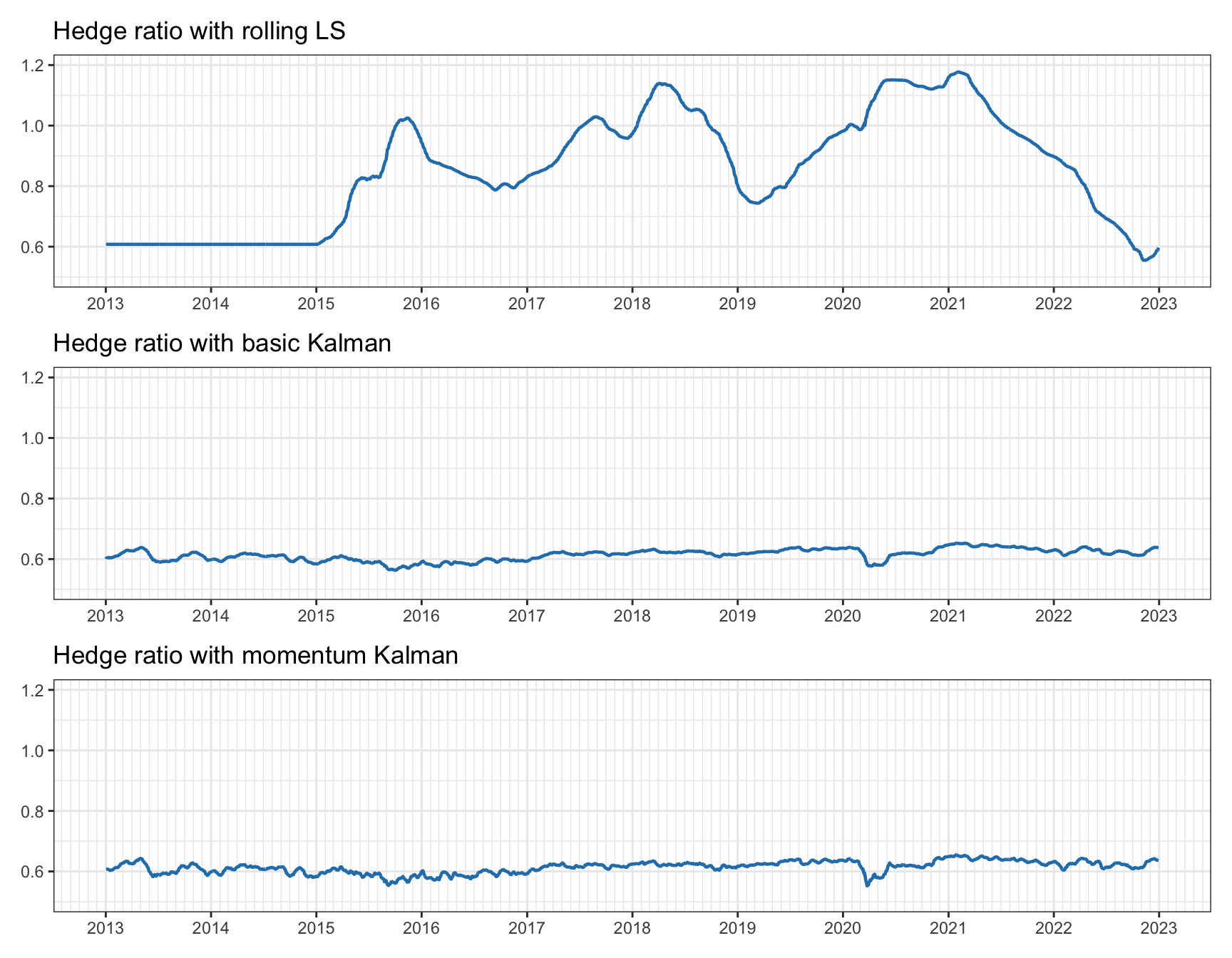
Figure 15.21: Tracking of hedge ratio for pairs trading on EWA–EWC.
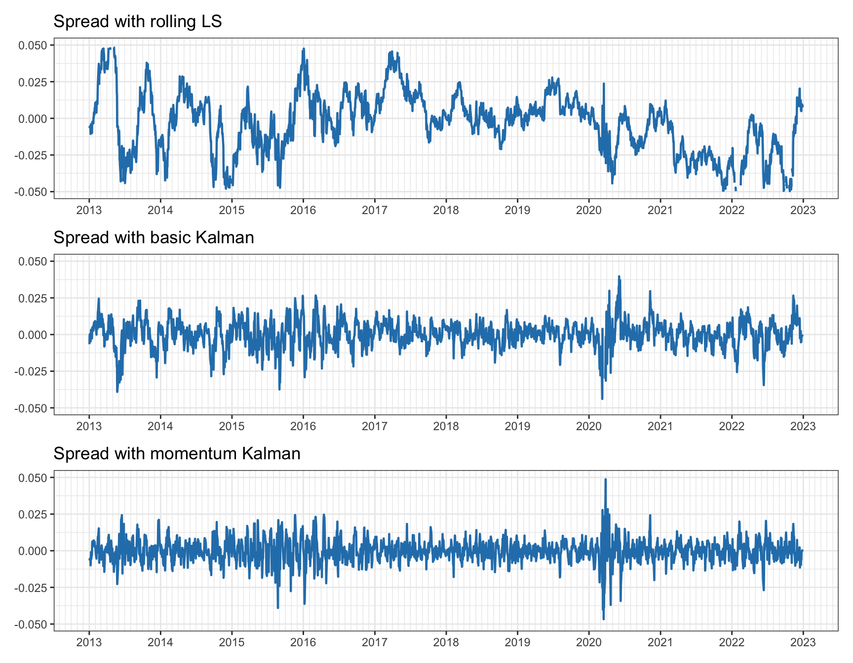
Figure 15.22: Spread for pairs trading on EWA–EWC.
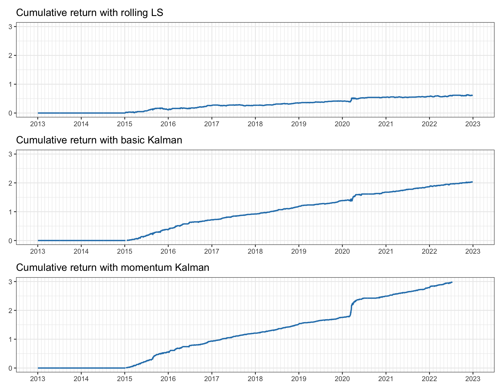
Figure 15.23: Cumulative return for pairs trading on EWA–EWC.
Market Data: KO and PEP
Next, we revisit pairs trading with the stocks Coca-Cola (KO) and Pepsi (PEP). As concluded from the cointegration tests in Section 15.4, they do not seem to be cointegrated. In addition, from the trading experiments in Section 15.5, profitability was dubious as indicated in Figures 15.19 and 15.18. We now look to see if the situation can be resolved with the Kalman-based methods.
Figure 15.24 shows the estimated hedge ratios over time. Again, we can observe that rolling least squares is noisy and not very consistent, whereas Kalman-based methods are stable while still being able to adapt to the big change that happens in early 2020 (perhaps due to the COVID-19 pandemic).
Figure 15.25 gives the spreads, and one can clearly appreciate a significant difference among the three methods. Observe early 2020: rolling least squares loses the tracking and cointegration is clearly lost, the basic Kalman is able to track after a momentary loss reflected in the shock on the spread, and the Kalman with momentum is able to track much better.
Finally, Figure 15.26 provides the cumulative returns, which gives a very clear picture. The difference among the three methods is quite astonishing. However, once more, one cannot forget that transaction costs have not been considered. In any case, the drawdown with Kalman-based methods is totally under control (unlike with rolling least squares). The conclusion is very clear: Kalman filtering is a must in pairs trading.
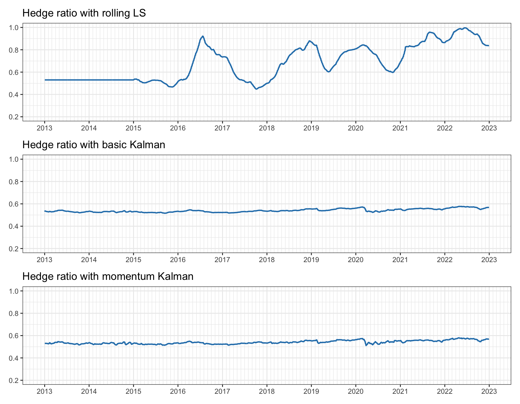
Figure 15.24: Tracking of hedge ratio for pairs trading on KO–PEP.
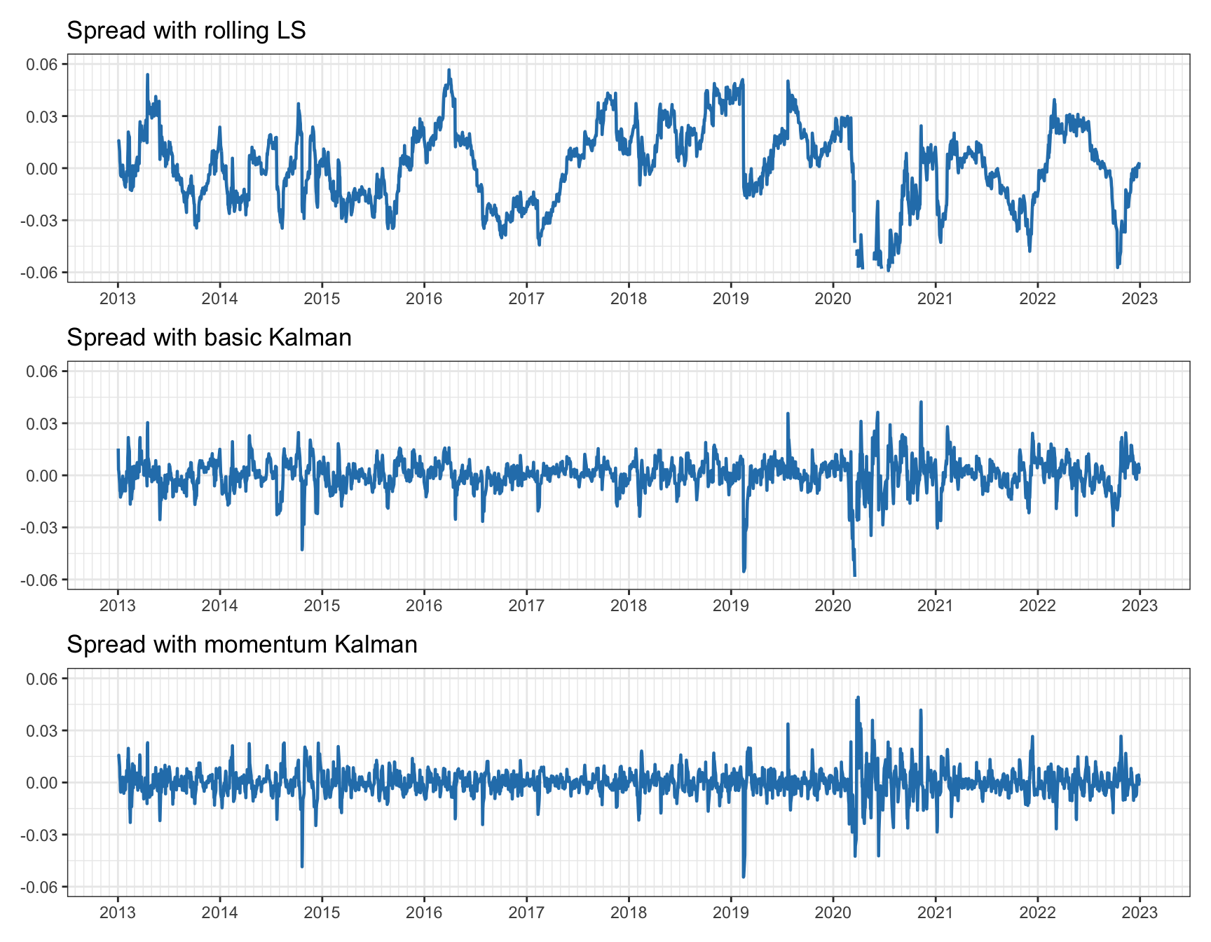
Figure 15.25: Spread for pairs trading on KO–PEP.
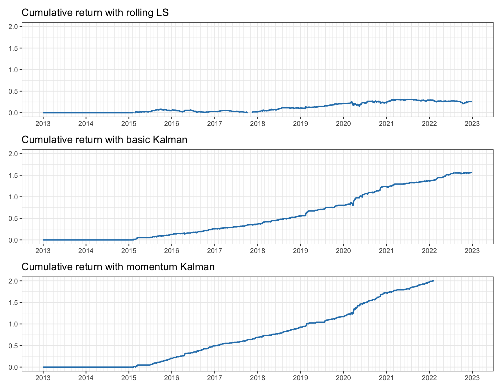
Figure 15.26: Cumulative return for pairs trading on KO–PEP.
References
The Kalman filter is implemented in the R package
KFAS(Helske, 2017) and the Python packagefilterpy. ↩︎The R package
MARSSimplements algorithms for fitting state-space models to time series data (Holmes et al., 2012). ↩︎