6.1 Fundamentals
6.1.1 Data Modeling
Following Chapters 2–4 on financial data modeling, we denote the prices of a universe of \(N\) assets by \(\bm{p}_t \in \R^N\), the linear returns by \[\bm{r}^{\textm{lin}}_t = \frac{\bm{p}_t - \bm{p}_{t-1}}{\bm{p}_{t-1}} = \frac{\bm{p}_t}{\bm{p}_{t-1}} - \bm{1},\] where the division is elementwise (with some abuse of notation), and the log-returns by \[\bm{r}^{\textm{log}}_t = \textm{log}\;\bm{p}_t - \textm{log}\;\bm{p}_{t-1},\] where the time index \(t\) can denote any arbitrary period such as minutes, hours, days, weeks, months, quarters, years, \(\ldots\)
The goal of the different financial data econometric models in Chapter 3, for the i.i.d. case, and Chapter 4, for time series with temporal structure, is to form a forecast or model for the returns at time \(t\) based on the previous historical data up to time \(t-1\), denoted by \(\mathcal{F}_{t-1}\). This modeling is typically done in terms of the conditional first- and second-order moments, that is, the conditional mean vector and covariance matrix: \[ \begin{aligned} \bmu^{\textm{log}}_{t} &\triangleq \E\left[\bm{r}^{\textm{log}}_{t} \mid \mathcal{F}_{t-1}\right],\\ \bSigma^{\textm{log}}_{t} &\triangleq \textm{Cov}\left[\bm{r}^{\textm{log}}_{t} \mid \mathcal{F}_{t-1}\right] = \E\left[\left(\bm{r}^{\textm{log}}_{t}-\bmu^{\textm{log}}_{t})(\bm{r}^{\textm{log}}_{t}-\bmu^{\textm{log}}_{t}\right)^\T \mid \mathcal{F}_{t-1}\right]. \end{aligned} \]
We remark that the majority of financial data models refer to the log-returns and not to the linear returns; for example, the random walk model for the log-prices in Chapter 3. However, to compute the return of a portfolio, from which its performance can be derived, it is the linear returns of the assets that are needed. This seems to create an impasse: we prefer to model the log-returns but what is really needed is the model of the linear returns.
In practice, since linear returns are very close to log-returns, \(\bm{r}^{\textm{lin}}_t \approx \bm{r}^{\textm{log}}_t\), for small values of the returns (see Chapter 2), most practitioners and academics simply use the following approximation and otherwise ignore the distinction between log- and linear returns: \[ \begin{aligned} \bmu^{\textm{lin}}_{t} &\approx \bmu^{\textm{log}}_{t},\\ \bSigma^{\textm{lin}}_{t} &\approx \bSigma^{\textm{log}}_{t}. \end{aligned} \] Mathematically, using the relationship between log-returns and linear returns, \(\bm{r}^{\textm{log}}_t = \textm{log}\big(\bm{1} + \bm{r}^{\textm{lin}}_t\big)\), or, equivalently, \(\bm{r}^{\textm{lin}}_t = \textm{exp}\big(\bm{r}^{\textm{log}}_t\big) - \bm{1}\), it follows that the mean vector and covariance matrix of the linear returns can be obtained from those of the log-returns as \[ \begin{aligned} \bmu^{\textm{lin}}_{t} &= \textm{exp}\left(\bmu^{\textm{log}}_t + \frac{1}{2}\textm{diag}\left(\bSigma^{\textm{log}}_t\right)\right) - \bm{1},\\ \left[\bSigma^{\textm{lin}}_{t}\right]_{ij} &= \left(\textm{exp}\left(\left[\bSigma^{\textm{log}}_{t}\right]_{ij}\right) - 1\right) \times\\ & \qquad\textm{exp}\left(\left[\bmu^{\textm{log}}_t\right]_i + \left[\bmu^{\textm{log}}_t\right]_j + \frac{1}{2}\left(\left[\bSigma^{\textm{log}}_{t}\right]_{ii} + \left[\bSigma^{\textm{log}}_{t}\right]_{jj}\right)\right). \end{aligned} \] However, due to the inherent noise in the estimation of the mean and covariance matrix, it is not clear that these more mathematically exact approximations give a practical advantage.
For the sake of notation, in the rest of the chapter we will drop the time dependency of the first- and second-order moments. In fact, in many cases the adopted econometric model is the i.i.d. one (see Chapter 3), which assumes no time dependency. In addition, we will refer to the linear moments by default: \[ \begin{aligned} \bmu &= \bmu^{\textm{lin}}_{t},\\ \bSigma &= \bSigma^{\textm{lin}}_{t}. \end{aligned} \]
6.1.2 Portfolio Return and Net Asset Value (NAV)
A portfolio is simply an allocation of the available budget among \(N\) risky assets (the amount not invested is kept as cash). The most common way to define a portfolio at time \(t\) is via its dollar allocation27 or capital allocation \(\w^\textm{cap}_t\in\R^N,\) where \(w^\textm{cap}_{i,t}\) denotes the dollar or capital amount allocated to the \(i\)th asset. Typically we denote the cash as a separate scalar \(c^\textm{cap}_t\in\R,\) although it is also possible to include it as part of the portfolio vector \(\w^\textm{cap}_t\) by considering it as one extra riskless asset (however, that would produce a singular covariance matrix, which may lead to numerical issues in the optimization part). Another way to represent a portfolio is via the number of units held for the assets \(\w^\textm{units}_t\in\R^N\); for example, in the case of a stock, a unit represents a share of a company and, in the case of a cryptocurrency, it represents a coin amount.
It is important to realize that if the unit amount is kept constant over time, \(\w_t^\textm{units}=\w^\textm{units}\), then the dollar amount will change as the prices of the assets change: \(\w^\textm{cap}_t = \w^\textm{units} \odot \bm{p}_t\).28 To be exact, the change in the portfolio is \[\begin{equation} \w^\textm{cap}_t = \w^\textm{cap}_{t-1} \odot \left(\bm{p}_t\oslash\bm{p}_{t-1}\right) = \w^\textm{cap}_{t-1} \odot \left(\bm{1} + \bm{r}^{\textm{lin}}_t\right), \tag{6.1} \end{equation}\] while the cash remains constant, \(c^\textm{cap}_t = c^\textm{cap}_{t-1}\), unless there is some cash contribution or withdrawal (negative contribution), in which case it would have to be reflected as \(c^\textm{cap}_t = c^\textm{cap}_{t-1} + \textm{contribution}_{t-1}\). If a fixed dollar amount over time is desired, \(\w^\textm{cap}_t = \w^\textm{cap}\), then the portfolio has to be regularly rebalanced, that is, the components of \(\w^\textm{cap}_t\) have to be adjusted (by buying or selling the assets) to bring them back to the originally designed positions, incurring in transaction costs. Figure 6.1 illustrates the change of the \(1/N\) portfolio over time until a rebalance is executed.
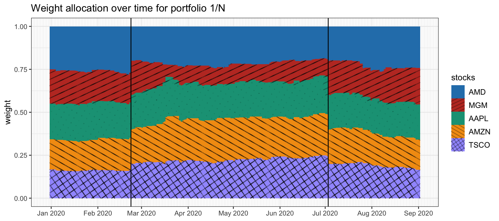
Figure 6.1: Evolution of the \(1/N\) portfolio over time with effect of rebalancing (vertical lines).
NAV and Return
The portfolio net asset value (NAV), commonly referred to as wealth, is defined as the value of the portfolio at the current market valuation including cash: \[\begin{equation} \textm{NAV}_t \triangleq \bm{1}^\T\w^\textm{cap}_t + c^\textm{cap}_t. \tag{6.2} \end{equation}\] Plugging the portfolio time evolution (6.1) into (6.2) gives the NAV evolution \[\begin{equation} \begin{aligned}[b] \textm{NAV}_t &= \bm{1}^\T\w^\textm{cap}_t + c^\textm{cap}_t\\ &= \bm{1}^\T\left(\w^\textm{cap}_{t-1} \odot \left(\bm{1} + \bm{r}^{\textm{lin}}_t\right)\right) + c^\textm{cap}_{t-1}\\ &= \textm{NAV}_{t-1} + \left(\w^{\textm{cap}}_{t-1}\right)^\T\bm{r}^{\textm{lin}}_t, \end{aligned} \tag{6.3} \end{equation}\] which indicates that the change in NAV depends on the assets’ returns and the portfolio via the term \(\big(\w^{\textm{cap}}_{t-1}\big)^\T\bm{r}^{\textm{lin}}_t\).
The portfolio return is then29 \[\begin{equation} R^\textm{portf}_t \triangleq \frac{\textm{NAV}_t - \textm{NAV}_{t-1}}{\textm{NAV}_{t-1}} = \w_{t-1}^\T\bm{r}^{\textm{lin}}_t, \tag{6.4} \end{equation}\] where \[\begin{equation} \w_{t} = \w^\textm{cap}_{t}/\textm{NAV}_{t} \tag{6.5} \end{equation}\] is the normalized portfolio with respect to the current NAV. In portfolio design or portfolio optimization, it is precisely the normalized version \(\w_{t}\) that is obtained. The expression \(\w_{t-1}^\T\bm{r}^{\textm{lin}}_t\) in (6.4) explains what is commonly referred to as the asset additivity property of the linear returns (as opposed to the time additivity property of the log-returns). Figure 6.2 shows the return and NAV of a portfolio over time.
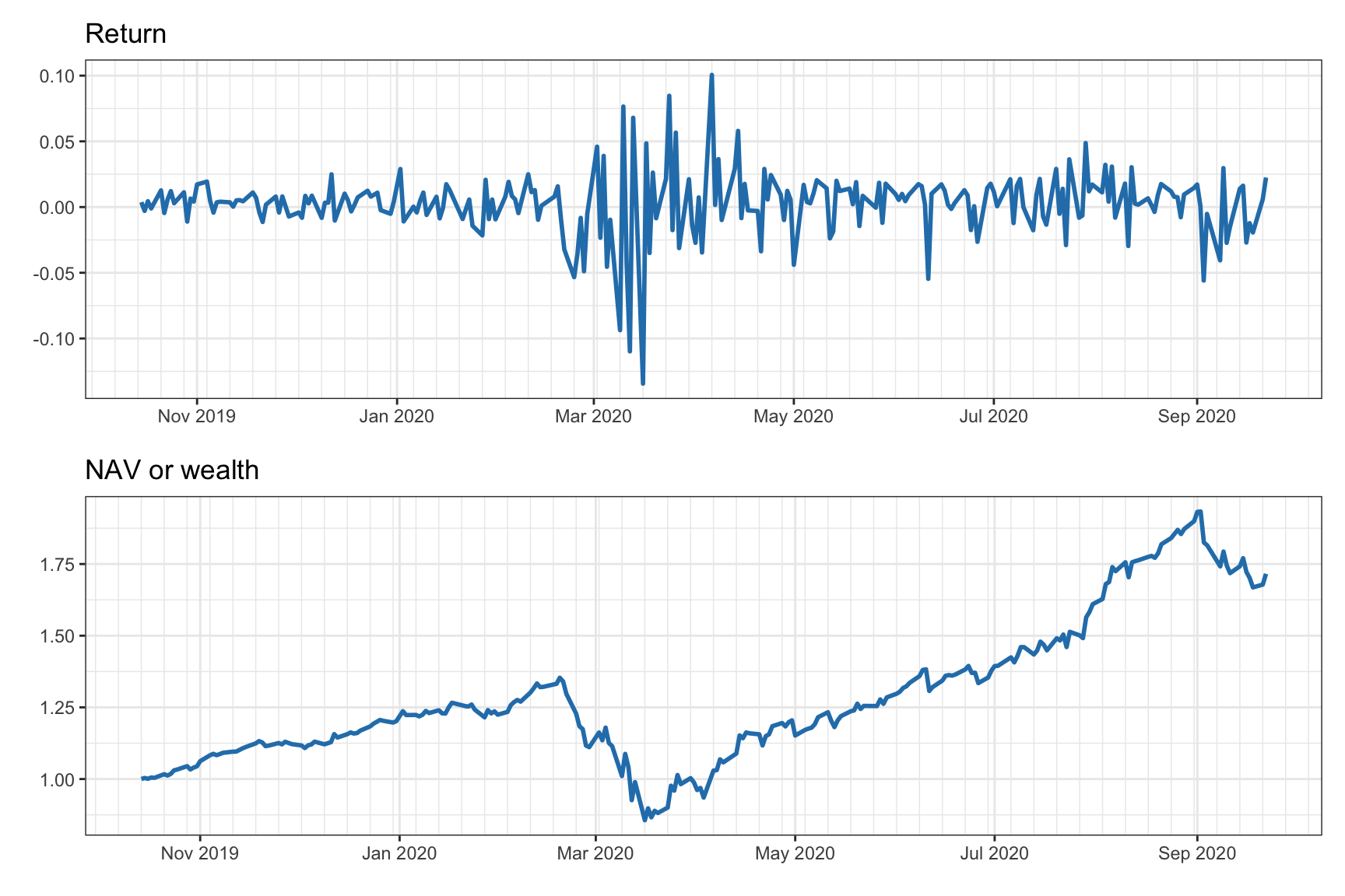
Figure 6.2: Return and NAV of the \(1/N\) portfolio over time.
Care has to be taken with the definition and implication of the time index, as illustrated in Figure 6.3. The portfolio at time \(t\) is \(\w_t\), which has used information up to time \(t-1\) (since that is the information used to estimate the moments \(\bmu_t\) and \(\bSigma_t\)) and executed at time \(t\).30 At this point, one might be tempted to obtain the return of the portfolio by multiplying the portfolio \(\w_t\) by the return at the same period \(\bm{r}^{\textm{lin}}_t\), but this would be incorrect as it would incur a look-ahead bias (refer to Chapter 8 for the dangers of backtesting). Since \(\w_t\) is the portfolio executed and held at time \(t\), with prices \(\bm{p}_t\), its return can be computed upon observing the prices \(\bm{p}_{t+1}\), that is, as \(\w_{t}^\T\bm{r}^{\textm{lin}}_{t+1}.\) Note that some authors instead define the returns with a shift in the time index so that \(\bm{p}_t\) can be multiplied by \(\bm{r}^{\textm{lin}}_{t}\).

Figure 6.3: Portfolio notation over time periods.
The first- and second-order moments of the portfolio return are key quantities in portfolio optimization. For a given portfolio, the expected value and variance of the portfolio return in (6.4) are given by \[ \begin{aligned} \E\left[R^\textm{portf}_t\right] &= \w_{t-1}^\T\bmu,\\ \textm{Var}\left[R^\textm{portf}_t\right] &= \w_{t-1}^\T\bSigma\w_{t-1}. \end{aligned} \]
6.1.3 Cumulative Return
The portfolio return at each given time \(t\) is a key quantity for assessing the portfolio performance. However, it is also invaluable to compute the cumulative return from inception to time \(t\), also referred to as cumulative profit and loss (P&L).
Essentially, the cumulative return is equivalent to the NAV (or wealth), except that it is normalized and the initial NAV (or budget) is subtracted as \(\textm{NAV}_t/\textm{NAV}_0 - 1\) (also, it does not account for contributions or redemptions related to the strategy). A plot of the cumulative return over time should start at zero, whereas a plot of the NAV or portfolio wealth starts at 1 (assuming it is normalized).
It is important to note that the cumulative return and NAV not only depend on the portfolio design at each period but also on the budget invested at each period (while some of the budget may remain as cash reserves). The amount of capital invested is often called position size. We now consider two extreme cases: full reinvesting and constant reinvesting.
Full reinvesting: Suppose we design a normalized portfolio \(\w_t\) and we fully reinvest the current NAV: \(\w^\textm{cap}_t = \textm{NAV}_{t}\times\w_t\). Then, the NAV evolution in (6.3) leads to \[ \textm{NAV}_t = \textm{NAV}_{t-1} + \textm{NAV}_{t-1}\times\w_{t-1}^\T\bm{r}^{\textm{lin}}_t = \textm{NAV}_{t-1} \times \left(1 + R^\textm{portf}_t\right), \] which corresponds to a geometric growth: \[\begin{equation} \textm{NAV}_t = \textm{NAV}_{0} \times \left(1 + R^\textm{portf}_1\right) \times \left(1 + R^\textm{portf}_2\right) \times \dots \times \left(1 + R^\textm{portf}_t\right). \tag{6.6} \end{equation}\]
Constant reinvesting: Now, suppose we design the same normalized portfolio \(\w_t\) but we keep reinvesting the same initial NAV: \(\w^\textm{cap}_t = \textm{NAV}_{0}\times\w_t\). Then, the NAV evolution in (6.3) leads to \[ \textm{NAV}_t = \textm{NAV}_{t-1} + \textm{NAV}_{0}\times\w_{t-1}^\T\bm{r}^{\textm{lin}}_t = \textm{NAV}_{t-1} + \textm{NAV}_{0}\times R^\textm{portf}_t, \] which corresponds to an arithmetic growth: \[\begin{equation} \textm{NAV}_t = \textm{NAV}_{0} \times \left(1 + R^\textm{portf}_1 + R^\textm{portf}_2 + \dots + R^\textm{portf}_t\right). \tag{6.7} \end{equation}\]
Figure 6.4 illustrates the difference between arithmetic and geometric cumulative returns: the shape of the curves is similar except that the swings are bigger for the geometric case. As previously mentioned, these curves start at 1, so strictly speaking they refer to the normalized NAV or wealth, while the cumulative returns should be shifted down to 0. This abuse of notation is understood in the financial context and no further comment or distinction will be made.
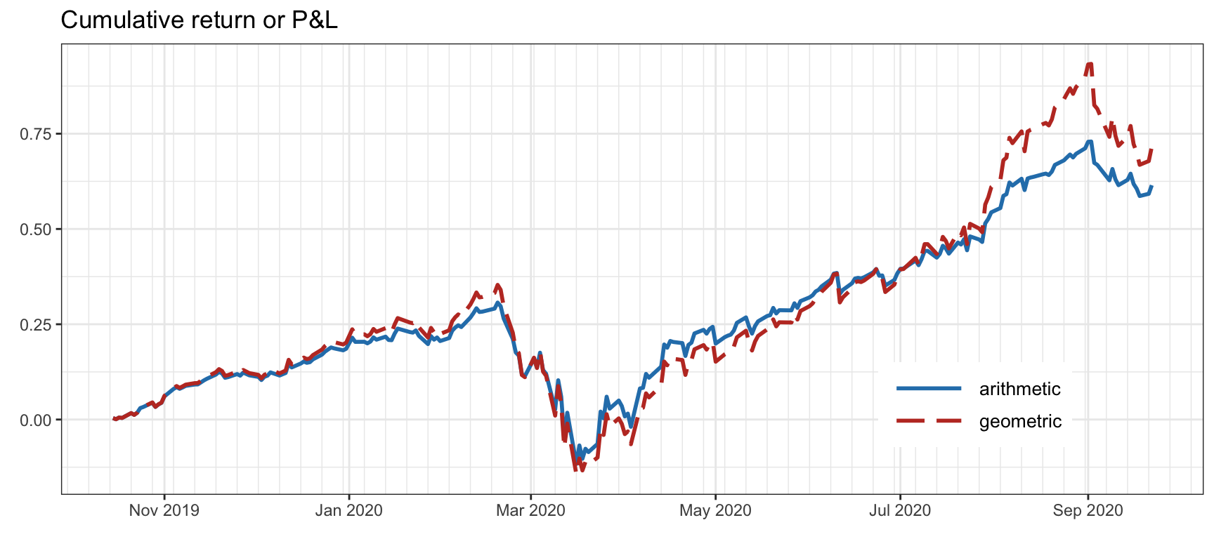
Figure 6.4: Comparison of arithmetic and geometric cumulative returns.
6.1.4 Transaction Costs
Every financial trade has an associated cost, called the transaction cost, that will diminish the overall return of the investment. Transaction costs consists of two terms: commission fee and slippage. The commission fee is the payment we make to our broker for completing the transaction. There is no universal scheme for commission fees: it depends on the country and the specific broker. For example, the U.S. in general has lower commission fees than European and Asian countries. Slippage refers to the difference between the expected price of a trade and the price at which the trade is actually executed. It does not directly refer to a negative or positive movement, as any change between the expected and actual prices can qualify. In general, liquid31 assets have smaller slippage than illiquid assets.
Suppose the current portfolio \(\w^\textm{cap}_t\) is rebalanced to \(\w^{\textm{cap},\textm{reb}}_t\). Then the portfolio NAV will decrease by the transaction cost, denoted by \(\phi\big(\w^\textm{cap}_t \rightarrow \w^{\textm{cap},\textm{reb}}_t\big)\). The notation details of the NAV computation may differ depending on whether the transaction cost is accounted after the price change or before. Calculating the NAV after the rebalancing and the price change, equation (6.1) is modified to \[ \begin{aligned} \textm{NAV}_t &= \bm{1}^\T\w^{\textm{cap}}_t + c^{\textm{cap}}_t\\ &= \bm{1}^\T\left(\w^{\textm{cap},\textm{reb}}_{t-1} \odot \left(\bm{1} + \bm{r}^{\textm{lin}}_t\right)\right) + c^{\textm{cap},\textm{reb}}_{t-1} - \phi\left(\w^{\textm{cap}}_{t-1} \rightarrow \w^{\textm{cap},\textm{reb}}_{t-1}\right)\\ &= \textm{NAV}_{t-1} + \big(\w^{\textm{cap},\textm{reb}}_{t-1}\big)^\T\bm{r}^{\textm{lin}}_t - \phi\left(\w^{\textm{cap}}_{t-1} \rightarrow \w^{\textm{cap},\textm{reb}}_{t-1}\right), \end{aligned} \] with the portfolio return then given by \[ R^\textm{portf}_t = \big(\w_{t-1}^{\textm{reb}}\big)^\T\bm{r}^{\textm{lin}}_t - \phi\left(\w_{t-1} \rightarrow \w_{t-1}^\textm{reb}\right), \] where the first term corresponds to the return due to the change of prices and the second term is the penalty due to transaction costs. Figure 6.5 shows the effect of transaction costs with daily rebalancing and 90 basis points (bps)32 of fees.
The expected value and variance of the portfolio return in this case are given by \[ \begin{aligned} \E\left[R^\textm{portf}_t\right] &= \left(\w^\textm{reb}_{t-1}\right)^\T\bmu - \phi\left(\w_{t-1} \rightarrow \w_{t-1}^\textm{reb}\right),\\ \textm{Var}\left[R^\textm{portf}_t\right] &= \left(\w^\textm{reb}_{t-1}\right)^\T\bSigma\w^\textm{reb}_{t-1}. \end{aligned} \]
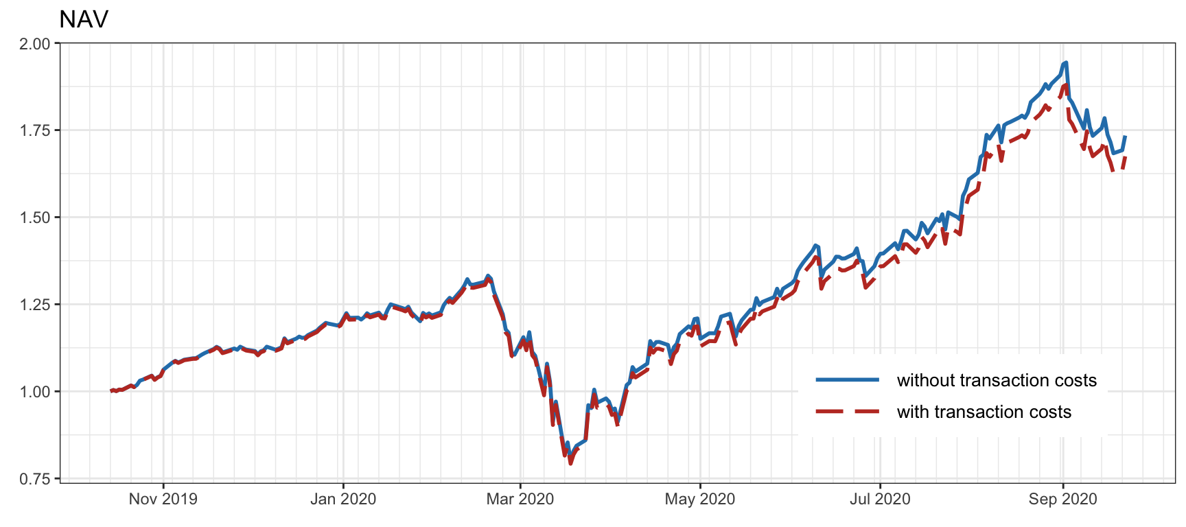
Figure 6.5: Effect of transaction costs on the NAV (with daily rebalancing and 90 bps of fees).
Let us focus on the form of the transaction cost function, which can be decomposed into fees and slippage: \[ \phi\left(\w_{t} \rightarrow \w_{t}^\textm{reb}\right) = \phi^\textm{fees}\left(\w_{t} \rightarrow \w_{t}^\textm{reb}\right) + \phi^\textm{slippage}\left(\w_{t} \rightarrow \w_{t}^\textm{reb}\right). \]
The details of \(\phi^\textm{fees}(\cdot)\) depend on the specific broker, but it can be approximated as being proportional to the turnover, \(\|\w_{t}^\textm{reb} - \w_{t}\|_1 = \sum_{i=1}^N |w_{it}^\textm{reb} - w_{it}|\), leading to \[ \phi^\textm{fees}\left(\w_{t} \rightarrow \w_{t}^\textm{reb}\right) \approx \tau^\textm{fee}\|\w_{t}^\textm{reb} - \w_{t}\|_1, \] where the fee factor \(\tau^\textm{fee}\) is typically around \(1--30\) bps. Keep in mind that some brokers include a minimum cost and may also have calculations based on shares instead of dollar amount.33
Let us consider the costs due to slippage, \(\phi^\textm{slippage}\left(\w_{t} \rightarrow \w_{t}^\textm{reb}\right)\). Slippage can also be approximated as proportional to the turnover (assuming that the liquidity is enough to absorb the order executed, otherwise it can significantly increase due to market impact), but the slippage will be different for each asset: \[ \phi^\textm{slippage}\left(\w_{t} \rightarrow \w_{t}^\textm{reb}\right) \approx \sum_{i=1}^N \tau_i^\textm{slippage}|w_{it}^\textm{reb} - w_{it}|, \] where \(\tau_i^\textm{slippage}\) is the asset-dependent slippage factor. In practice, the slippage factor can be estimated from the bid–ask spread of an asset. Although one can find various models to estimate slippage, a simple one is the following: \[ \tau^\textm{slippage} = \frac{\textm{half of spread}}{\textm{middle of spread}} = \frac{0.5(\textm{bid} - \textm{ask})}{0.5(\textm{bid} + \textm{ask})} = \frac{\textm{bid} - \textm{ask}}{\textm{bid} + \textm{ask}}. \]
When assessing the performance of a portfolio via backtests, it is recommended to account for transaction costs to get a more realistic result, as shown in Figure 6.5. Since the transaction costs depend on the turnover, it also important to monitor the turnover of the strategy or related measures such as return on turnover.
6.1.5 Portfolio Rebalancing
Since rebalancing a portfolio entails transaction costs, there is a fundamental trade-off: we should rebalance the portfolio frequently (so as to match the currently held portfolio in the market with the desired one) but not that frequently in order to keep the transaction costs low.
The simplest way to rebalance a portfolio is with a regular calendar-based scheme, such as daily, weekly, or monthly rebalancing. There are other rebalancing schemes that decide whether to rebalance in an adaptive fashion; for example, rebalance \(\w_{t} \rightarrow \w_{t}^\textm{reb}\) only if their distance is above some small threshold, which is used to ignore unnecessary rebalancing due to errors in the estimation and portfolio design process. Some common ways to measure the difference between portfolios include the turnover \(\|\w_{t}^\textm{reb} - \w_{t}\|_1\) or some measure of statistical difference such as the squared Mahalanobis distance \((\w_{t}^\textm{reb} - \w_{t})^\T\bSigma^{-1}(\w_{t}^\textm{reb} - \w_{t})\) (Scherer, 2002) or the tracking error squared distance \((\w_{t}^\textm{reb} - \w_{t})^\T\bSigma(\w_{t}^\textm{reb} - \w_{t})\) widely used in asset management (Michaud and Michaud, 2008), where \(\bSigma\) denotes the covariance matrix of the assets. At the same time, the turnover \(\|\w_{t}^\textm{reb} - \w_{t}\|_1\) is typically upper-bounded or penalized in the portfolio design process to avoid frequent and large rebalancing.
The portfolio time-index notation illustrated in Figure 6.3 does not take into account the portfolio rebalancing process. To properly reflect that, the notation necessarily becomes more involved. A common way is to refine the notation by considering that each period \(t\) can be divided into the beginning of period (bop) and the end of period (eop); for example, the portfolio \(\w_{t}\) can be more finely separated into \(\w^\textm{bop}_{t}\) and \(\w^\textm{eop}_{t}\), as shown in Figure 6.6.

Figure 6.6: Portfolio notation over time periods with rebalancing.
According to this notation, the change from \(\w^\textm{bop}_{t}\) to \(\w^\textm{eop}_{t}\) is due to the price change as in (6.1), \[ \w^\textm{eop}_{t} = \w^\textm{bop}_{t} \odot \left(\bm{1} + \bm{r}^{\textm{lin}}_t\right), \] and the change from \(\w^\textm{eop}_{t}\) to \(\w^\textm{bop}_{t+1}\) is due to the rebalancing which incurs a transaction cost (if there is no rebalancing, then simply \(\w^\textm{bop}_{t+1}=\w^\textm{eop}_{t}\)). For example, suppose that we rebalance a fixed portfolio \(\w\) at each period \(t\) and ignore the transaction cost; then, the portfolio after rebalancing is \(\w^\textm{bop}_{t}=\w\), after the prices change it becomes \(\w^\textm{eop}_{t} = \w^\textm{bop}_{t} \odot \left(\bm{1} + \bm{r}^{\textm{lin}}_t\right)\), and the portfolio return from (6.4) is \[\begin{equation} R^\textm{portf}_t = \w^\T\bm{r}^{\textm{lin}}_t. \tag{6.8} \end{equation}\]
Figure 6.7 illustrates the effect of different reoptimization and rebalancing schemes with transaction costs of 20 bps (rebalancing refers to executing the desired portfolio in the market, whereas reoptimization refers to collecting new data, estimating the mean and covariance matrix, and solving an optimization problem to design a new portfolio).
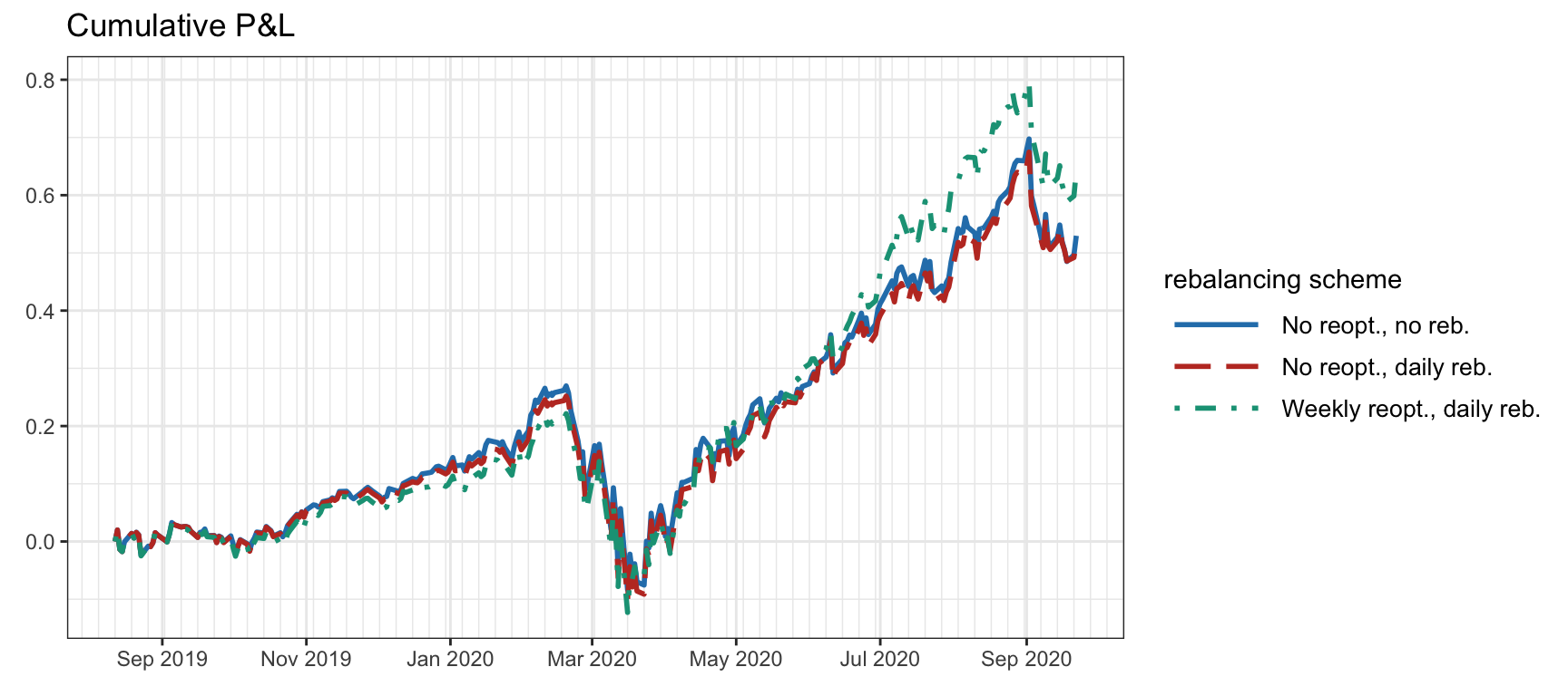
Figure 6.7: Backtest cumulative P&L of a portfolio with different reoptimization and rebalancing schemes.
References
The term “dollar” is an abuse of terminology and it can, of course, refer to any currency, such as the Euro, or even a cryptocurrency, such as Bitcoin.↩︎
For convenience of notation, we denote the elementwise product between vectors by \(\odot\) and elementwise division by \(\oslash\).↩︎
Note that if there have been cash constributions, they have to be removed in the computation of the portfolio return: \(R^\textm{portf}_t \triangleq (\textm{NAV}_t - \textm{NAV}_{t-1} - \textm{contribution}_{t-1})/\textm{NAV}_{t-1} = \w_{t-1}^\T\bm{r}^{\textm{lin}}_t\).↩︎
It could be argued that it might be possible to execute the portfolio instantaneously after observing the data at time \(t-1\), although that would imply an instantaneous (or sufficiently fast) forecast, portfolio design, and market execution.↩︎
Liquidity refers to the efficiency or ease with which an asset or security can be converted into ready cash without affecting its market price. The most liquid asset of all is cash itself.↩︎
Basis points, denoted by bps, represents a factor of \(10^{-4}\). For example, 16 bps means 0.0016 or 0.16%.↩︎
Fees of popular broker dealer Interactive Brokers: www.interactivebrokers.com↩︎