9.2 High-Order Moments
The first two moments of a random variable are enough to characterize its distribution only if it follows a Gaussian or normal distribution; otherwise, higher-order moments, also termed higher-order statistics, are necessary.
The first four moments of a random variable \(X\) are
- the mean or first moment (measure of location): \(\bar{X} \triangleq \E\left[X\right]\);
- the variance or second central moment (measure of dispersion): \(\E[(X - \bar{X})^2]\);
- the skewness44 or third central moment (measure of asymmetry): \(\E[(X - \bar{X})^3]\); and
- the kurtosis45 or fourth central moment (measure of thickness of tails): \(\E[(X - \bar{X})^4]\).
Next, we explore the expressions of the high-order statistics for the portfolio return.
9.2.1 Nonparametric Case
In the portfolio context with a universe of \(N\) assets, we denote by \(\bm{r}\in\R^N\) the returns of the \(N\) assets and by \(\w\in\R^N\) the portfolio weights. Then, the return of this portfolio is \(\w^\T\bm{r}\) and the first four moments are given by \[\begin{equation} \begin{aligned} \phi_1(\w) & \triangleq \E\left[\w^\T\bm{r}\right] = \w^\T\bmu,\\ \phi_2(\w) & \triangleq \E\left[\left(\w^\T\bm{\bar{r}}\right)^2\right] = \w^\T\bSigma\w,\\ \phi_3(\w) & \triangleq \E\left[\left(\w^\T\bm{\bar{r}}\right)^3\right] = \w^\T\bm{\Phi}(\w\otimes\w),\\ \phi_4(\w) & \triangleq \E\left[\left(\w^\T\bm{\bar{r}}\right)^4\right] = \w^\T\bm{\Psi}(\w\otimes\w\otimes\w), \end{aligned} \tag{9.1} \end{equation}\] where \(\bmu = \E[\bm{r}] \in \R^N\) is the mean vector, \(\bm{\bar{r}} = \bm{r} - \bmu\) are the centered returns, \(\bSigma = \E\left[\bm{\bar{r}}\bm{\bar{r}}^\T\right] \in \R^{N\times N}\) is the covariance matrix, \(\bm{\Phi} = \E\left[\bm{\bar{r}}(\bm{\bar{r}}\otimes\bm{\bar{r}})^\T\right] \in \R^{N\times N^2}\) is the co-skewness matrix, and \(\bm{\Psi} = \E\left[\bm{\bar{r}}(\bm{\bar{r}}\otimes\bm{\bar{r}}\otimes\bm{\bar{r}})^\T\right] \in \R^{N\times N^3}\) is the co-kurtosis matrix.
The gradients and Hessians of the moments, required by numerical algorithms, are given by \[\begin{equation} \begin{aligned} \nabla\phi_1(\w) &= \bmu,\\ \nabla\phi_2(\w) &= 2\,\bSigma\w,\\ \nabla\phi_3(\w) &= 3\,\bm{\Phi}(\w\otimes\w),\\ \nabla\phi_4(\w) &= 4\,\bm{\Psi}(\w\otimes\w\otimes\w)\\ \end{aligned} \tag{9.2} \end{equation}\] and \[\begin{equation} \begin{aligned} \nabla^2\phi_1(\w) &= \bm{0},\\ \nabla^2\phi_2(\w) &= 2\,\bSigma,\\ \nabla^2\phi_3(\w) &= 6\,\bm{\Phi}(\bm{I}\otimes\w),\\ \nabla^2\phi_4(\w) &= 12\,\bm{\Psi}(\bm{I}\otimes\w\otimes\w), \end{aligned} \tag{9.3} \end{equation}\] respectively (Zhou and Palomar, 2021).
Complexity Analysis
The main problem with high-order moments is the sheer number of elements required to characterize them. This has direct implications on the computational cost, as well as the memory cost.
To simplify the analysis, rather than characterizing the exact cost or complexity, we are just interested in how the complexity grows with the dimensionality \(N\). This can be done with the “big O” notation, which measures the order of complexity. To be specific, we say that the complexity is \(f(N) = \bigO\left(g(N)\right)\), as \(N\rightarrow\infty\), if there exists a positive real number \(M\) and \(N_0\) such that \(|f(N)| \leq Mg(N)\) for all \(N\geq N_0\).
Let us start by looking at the four parameters \(\bmu\), \(\bSigma\), \(\bm{\Phi}\), and \(\bm{\Psi}\). From their dimensions, we can infer that their complexity is \(\bigO(N)\), \(\bigO(N^2)\), \(\bigO(N^3)\), and \(\bigO(N^4)\), respectively. The computation of the portfolio moments in (9.1) has the same complexity order. Regarding the gradients in (9.2), their computation has complexity \(\bigO(1)\), \(\bigO(N^2)\), \(\bigO(N^3)\), and \(\bigO(N^4)\), respectively. Finally, the complexity of the computation of the Hessians in (9.3) is \(\bigO(1)\), \(\bigO(1)\), \(\bigO(N^3)\), and \(\bigO(N^4)\), respectively.
For example, when \(N=200\), storing the co-kurtosis matrix \(\bm{\Psi}\) requires almost 12\(\,\)GB of memory (assuming a floating-point number is represented with 64 bits or 8 bytes).
Summarizing, while the complexity order of the first and second moments in Markowitz’s portfolio is \(\bigO(N^2)\), further incorporating the third and fourth moments increases the complexity order to \(\bigO(N^4)\), which severely limits the practical application to scenarios with small number of assets.
9.2.2 Structured Moments
One way to reduce the number of parameters to be estimated in the high-order moments is by introducing some structure in the high-order moment matrices via factor modeling (see Chapter 3). This will, however, make the estimation process much more complicated due to the intricate structure in the matrices.
Consider a single market-factor model of the returns, \[ \bm{r}_t = \bm{\alpha} + \bm{\beta} r^\textm{mkt}_t + \bm{\epsilon}_t, \] where \(\bm{\alpha}\) and \(\bm{\beta}\) are the so-called “alpha” and “beta,” respectively, \(r^\textm{mkt}_t\) is the market index, and \(\bm{\epsilon}_t\) the residual. Then, the moments can be written (Martellini and Ziemann, 2010) as \[\begin{equation} \begin{aligned} \bmu & = \bm{\alpha} + \bm{\beta} \phi^\textm{mkt}_1,\\ \bSigma & = \bm{\beta}\bm{\beta}^\T \phi^\textm{mkt}_2 + \bSigma_\epsilon,\\ \bm{\Phi} & = \bm{\beta}\left(\bm{\beta}^\T \otimes \bm{\beta}^\T\right) \phi^\textm{mkt}_3 + \bm{\Phi}_\epsilon,\\ \bm{\Psi} & = \bm{\beta}\left(\bm{\beta}^\T \otimes \bm{\beta}^\T \otimes \bm{\beta}^\T\right) \phi^\textm{mkt}_4 + \bm{\Psi}_\epsilon, \end{aligned} \tag{9.4} \end{equation}\] where \(\phi^\textm{mkt}_i\) denotes the \(i\)th moment of the market factor, and \(\bSigma_\epsilon\), \(\bm{\Phi}_\epsilon\), and \(\bm{\Psi}_\epsilon\) are the covariance, co-skewness, and co-kurtosis matrices of the residuals \(\bm{\epsilon}_t\), respectively.
Alternatively, we can assume a multi-factor model of the returns, \[ \bm{r}_t = \bm{\alpha} + \bm{B} \bm{f}_t + \bm{\epsilon}_t, \] where \(\bm{f}_t\in\R^K\) contains the \(K\) factors (typically with \(K\ll N\)). Then, the moments can be written (Boudt et al., 2014) as \[\begin{equation} \begin{aligned} \bmu & = \bm{\alpha} + \bm{B} \bm{\phi}^\textm{factors}_1,\\ \bSigma & = \bm{\beta}\bm{\Phi}^\textm{factors}_2\bm{\beta}^\T + \bSigma_\epsilon,\\ \bm{\Phi} & = \bm{\beta}\bm{\Phi}^\textm{factors}_3\left(\bm{\beta}^\T \otimes \bm{\beta}^\T\right) + \bm{\Phi}_\epsilon,\\ \bm{\Psi} & = \bm{\beta}\bm{\Phi}^\textm{factors}_4\left(\bm{\beta}^\T \otimes \bm{\beta}^\T \otimes \bm{\beta}^\T\right) + \bm{\Psi}_\epsilon, \end{aligned} \tag{9.5} \end{equation}\] where \(\bm{\phi}^\textm{factors}_1\) denotes the mean, and \(\bm{\Phi}^\textm{factors}_2\), \(\bm{\Phi}^\textm{factors}_3\), and \(\bm{\Phi}^\textm{factors}_4\), the covariance matrix, co-skewness matrix, and co-kurtosis matrix of the multiple factors in \(\bm{f}_t\), respectively.
In addition to the structure provided by factor modeling, another technique is via shrinkage, see Martellini and Ziemann (2010) and Boudt, Cornilly, and Verdonck (2020).
9.2.3 Parametric Case
Multivariate Normal Distribution
A multivariate normal (or Gaussian) distribution with mean \(\bmu\) and covariance matrix \(\bSigma\) is characterized by the probability density function \[ f_\textm{mvn}(\bm{x}) = \frac{1}{\sqrt{(2\pi)^N|\bSigma|}} \textm{exp}\left(-\frac{1}{2}(\bm{x} - \bmu)^\T\bSigma^{-1}(\bm{x} - \bmu)\right). \] A random vector \(\bm{x}\) drawn from the normal distribution \(f_\textm{mvn}(\bm{x})\) is denoted by \[ \bm{x} \sim \mathcal{N}(\bmu, \bSigma). \]
Nevertheless, decades of empirical studies have clearly demonstrated that financial data do not follow a Gaussian distribution (see Chapter 2 for stylized facts of financial data). Thus, we need more general distributions that can model the skewness (i.e., asymmetry) and kurtosis (i.e., heavy tails).
Multivariate Normal Mixture Distributions
The multivariate normal can be generalized to obtain multivariate normal mixture distributions. The crucial idea is the introduction of randomness into first the covariance matrix and then the mean vector of a multivariate normal distribution via a positive mixing variable, denoted by \(w\) (McNeil et al., 2015).
A multivariate normal variance mixture can be represented as \[ \bm{x} = \bmu + \sqrt{w}\bm{z}, \] where \(\bmu\) is referred to as the location vector, \(\bm{z} \sim \mathcal{N}(\bm{0}, \bSigma)\) with \(\bSigma\) referred to as the scatter matrix, and \(w\) is a nonnegative scalar-valued random variable independent of \(\bm{z}\). Observe that the random variable \(w\) only affects the covariance matrix, but not the mean, \[ \begin{aligned} \E[\bm{x}] &= \bmu,\\ \textm{Cov}(\bm{x}) &= \E[w]\bSigma, \end{aligned} \] hence the name variance mixture.
One important example of a normal variance mixture is the multivariate \(t\) distribution, obtained when \(w\) follows an inverse gamma distribution \(w \sim \textm{Ig}\left(\frac{\nu}{2}, \frac{\nu}{2}\right)\), which is equivalent to saying that \(\tau=1/w\) follows a gamma distribution \(\tau \sim \textm{Gamma}\left(\frac{\nu}{2}, \frac{\nu}{2}\right)\).46 This can be represented in a hierarchical structure as \[ \begin{aligned} \bm{x} \mid \tau &\sim \mathcal{N}\left(\bmu, \frac{1}{\tau}\bSigma\right),\\ \tau &\sim \textm{Gamma}\left(\frac{\nu}{2}, \frac{\nu}{2}\right). \end{aligned} \]
The multivariate \(t\) distribution (also called Student’s \(t\) distribution) is widely used to model heavy tails (via the parameter \(\nu\)) in finance and other areas. However, it cannot capture the asymmetries observed in financial data.
A more general case of normal variance mixture is the multivariate symmetric generalized hyperbolic distribution, obtained when \(w\) follows a generalized inverse Gaussian (GIG) distribution, which contains the inverse gamma distribution as a particular case. But this distribution still cannot capture asymmetries since it is a variance mixture. In order to model asymmetry, the mixture has to affect the mean as well.
A multivariate normal mean–variance mixture can be represented as \[ \bm{x} = \bm{m}(w) + \sqrt{w}\bm{z}, \] where \(\bm{m}(w)\) is now some function of \(w\) and the rest is as before for variance mixtures. A typical example of \(\bm{m}(w)\) is \(\bm{m}(w) = \bmu + w\bm{\gamma}\), leading to \[ \begin{aligned} \E[\bm{x}] &= \bmu + \E[w]\bm{\gamma},\\ \textm{Cov}(\bm{x}) &= \E[w]\bSigma + \textm{var}(w)\bm{\gamma}\bm{\gamma}^\T. \end{aligned} \]
An example of a mean–variance mixture is the multivariate generalized hyperbolic (GH) distribution, obtained when \(\bm{m}(w) = \bmu + w\bm{\gamma}\) and \(w\) follows a GIG distribution. If the GIG distribution is further particularized to an inverse gamma distribution, then the multivariate skewed \(t\) distribution (or generalized hyperbolic multivariate skewed \(t\) (ghMST)) is obtained, which can be conveniently represented in a hierarchical structure as \[ \begin{aligned} \bm{x} \mid \tau &\sim \mathcal{N}\left(\bmu + \frac{1}{\tau}\bm{\gamma}, \frac{1}{\tau}\bSigma\right),\\ \tau &\sim \textm{Gamma}\left(\frac{\nu}{2}, \frac{\nu}{2}\right). \end{aligned} \]
Other distributions more general than the ghMST could be considered, such as the restricted multivariate skewed \(t\) (rMST) distribution and the unrestricted multivariate skewed \(t\) (uMST) distribution; see X. Wang et al. (2023) and references therein for more details. However, these more complex distributions are significantly more complicated to fit to data (e.g., the uMST can only be fitted for \(N<10\) in practice due to the computational complexity) and do not seem to provide any advantage in modeling the asymmetries of financial data. Figure 9.2 shows the goodness of fit (via the out-of-sample likelihood of the fit) of several multivariate distributions from the simplest Gaussian to the most complicated uMST. The skewed \(t\) distribution seems to obtain a good fit while preserving its simplicity.
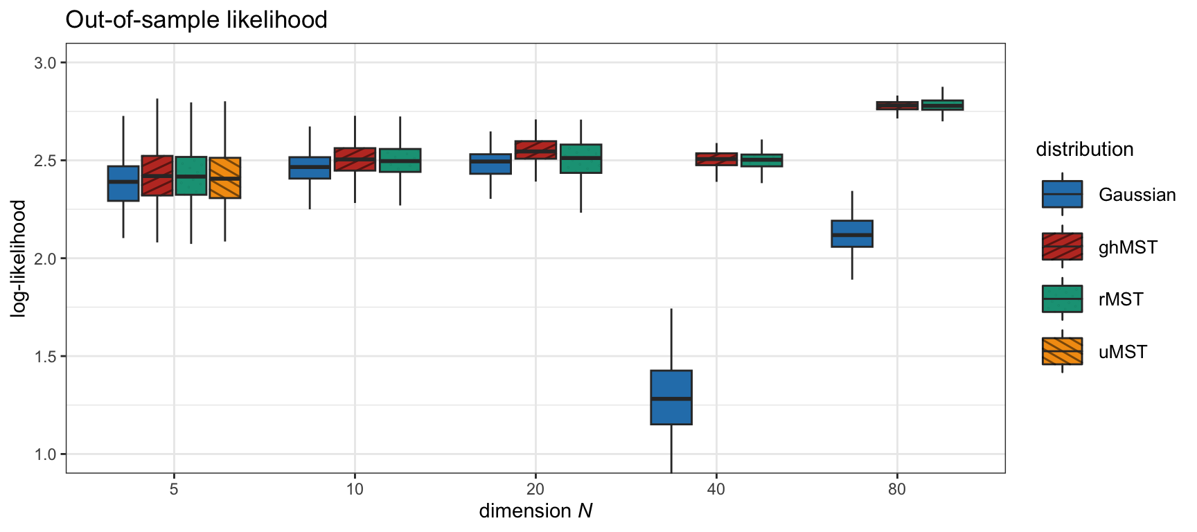
Figure 9.2: Likelihood of different fitted multivariate distributions for S&P 500 daily stock returns.
Parametric Moments
The advantage of assuming a parametric model for the data is that the computation of the moments simplifies a great deal. To be specific, under the multivariate skewed \(t\) distribution, the first four moments are conveniently simplified (Birgeand and Chavez-Bedoya, 2016; X. Wang et al., 2023) to \[\begin{equation} \begin{aligned} \phi_1(\w) & = \w^\T\bmu + a_1 \w^\T\bm{\gamma},\\ \phi_2(\w) & = a_{21}\w^\T\bSigma\w + a_{22}(\w^\T\bm{\gamma})^2,\\ \phi_3(\w) & = a_{31}(\w^\T\bm{\gamma})^3 + a_{32}(\w^\T\bm{\gamma})\w^\T\bSigma\w,\\ \phi_4(\w) & = a_{41}(\w^\T\bm{\gamma})^4 + a_{42}(\w^\T\bm{\gamma})^2\w^\T\bSigma\w + a_{43}(\w^\T\bSigma\w)^2, \end{aligned} \tag{9.6} \end{equation}\] where \(a_1=\frac{\nu}{\nu-2}\), \(a_{21}=a_1\), \(a_{22}=\frac{2\nu^2}{(\nu-2)^2(\nu-4)}\), \(a_{31}=\frac{16\nu^3}{(\nu-2)^3(\nu-4)(\nu-6)}\), \(a_{32}=\frac{6\nu^2}{(\nu-2)^2(\nu-4)}\), \(a_{41}=\frac{(12\nu+120)\nu^4}{(\nu-2)^4(\nu-4)(\nu-6)(\nu-8)}\), \(a_{42}=\frac{6(2\nu+4)\nu^3}{(\nu-2)^3(\nu-4)(\nu-6)}\), and \(a_{43}=\frac{3\nu^2}{(\nu-2)(\nu-4)}\).
It is important to emphasize that now \(\bmu\) refers to the location vector and not the mean; similarly, \(\bSigma\) now refers to the scatter matrix and not the covariance matrix.
The gradients and Hessians are given by \[\begin{equation} \begin{aligned} \nabla\phi_1(\w) &= \bmu + a_1 \bm{\gamma},\\ \nabla\phi_2(\w) &= 2a_{21}\bSigma\w + 2a_{22}(\w^\T\bm{\gamma})\bm{\gamma},\\ \nabla\phi_3(\w) &= 3a_{31}(\w^\T\bm{\gamma})^2\bm{\gamma} + a_{32}\left((\w^\T\bSigma\w)\bm{\gamma} + 2(\w^\T\bm{\gamma})\bSigma\w\right),\\ \nabla\phi_4(\w) &= 4a_{41}(\w^\T\bm{\gamma})^3\bm{\gamma}\\ &\quad + 2a_{42}\left((\w^\T\bm{\gamma})^2\bSigma\w + (\w^\T\bSigma\w)(\w^\T\bm{\gamma})\bm{\gamma}\right) + 4a_{43}(\w^\T\bSigma\w)\bSigma\w\\ \end{aligned} \tag{9.7} \end{equation}\] and \[\begin{equation} \begin{aligned} \nabla^2\phi_1(\w) &= \bm{0},\\ \nabla^2\phi_2(\w) &= 2a_{21}\bSigma + 2a_{22}\bm{\gamma}\bm{\gamma}^\T,\\ \nabla^2\phi_3(\w) &= 6a_{31}(\w^\T\bm{\gamma})\bm{\gamma}\bm{\gamma}^\T + 2a_{32}\left(\bm{\gamma}\w^\T\bSigma + \bSigma\w\bm{\gamma}^\T + (\w^\T\bm{\gamma})\bSigma\right),\\ \nabla^2\phi_4(\w) &= 12a_{41}(\w^\T\bm{\gamma})^2\bm{\gamma}\bm{\gamma}^\T\\ &+ 2a_{42}\left(2(\w^\T\bm{\gamma})\bSigma\w\bm{\gamma}^\T + (\w^\T\bm{\gamma})^2\bSigma + 2(\w^\T\bm{\gamma})\bm{\gamma}\w^\T\bSigma + (\w^\T\bSigma\w)\bm{\gamma}\bm{\gamma}^\T\right)\\ &+ 4a_{43}\left(2\bSigma\w\w^\T\bSigma + (\w^\T\bSigma\w)\bSigma\right), \end{aligned} \tag{9.8} \end{equation}\] respectively (X. Wang et al., 2023).
9.2.4 L-Moments
One property of higher-order moments is that they fully characterize the distribution function of the random variable. In addition, the first four moments convey descriptive properties of the random variable such as location, dispersion, asymmetry, and thickness of tails.
Interestingly, the so-called “L-moments” also characterize the distribution of a random variable and similarly convey descriptive properties (Hosking, 1990). In addition, they are linear functions of the order statistics and are easier to estimate in practice.
Let \(X\) be a random variable and \(X_{1:n} \leq X_{2:n} \leq \dots \leq X_{n:n}\) be the order statistics of a random sample of size \(n\) drawn from the distribution of \(X\). The L-moments of \(X\) are defined as \[ \lambda_r = \frac{1}{r}\sum_{k=0}^{r-1}(-1)^k\binom{r-1}{k}\E[X_{r-k:r}],\quad r=1,2,\dots \]
In particular, the first four L-moments are \[\begin{equation} \begin{aligned} \lambda_1 &= \E[X],\\ \lambda_2 &= \frac{1}{2}\E[X_{2:2} - X_{1:2}],\\ \lambda_3 &= \frac{1}{3}\E[X_{3:3} - 2 X_{2:3} + X_{1:3}]\\ &= \frac{1}{3}\E[(X_{3:3} - X_{2:3}) - (X_{2:3} - X_{1:3})],\\ \lambda_4 &= \frac{1}{4}\E[X_{4:4} - 3 X_{3:4} + 3 X_{2:4} - X_{1:4}]\\ &= \frac{1}{4}\E[(X_{4:4} - X_{1:4}) - 3(X_{3:4} - X_{2:4})]. \end{aligned} \tag{9.9} \end{equation}\] These moments provide descriptive information similar to the regular moments (Hosking, 1990):
- The L-location, \(\lambda_1\), is identical to the mean \(\bar{X}\).
- The L-scale, \(\lambda_2\), measures the expected difference between any two realizations. It resembles the variance expressed as \(\sigma^2=\frac{1}{2}\E[(X_{2:2} - X_{1:2})^2]\).
- The L-skewness, \(\lambda_3\), is the expected difference of differences. It provides a measure of the asymmetry less sensitive to extreme tails than the regular skewness \(\E[(X - \bar{X})^3]\), which makes its estimation more accurate in practice.
- The L-kurtosis, \(\lambda_4\), measures the expected exceedance of the largest difference. It is a measure of how thick the tails are, similar to the regular kurtosis \(\E[(X - \bar{X})^4]\), but, again, less sensitive to extreme tails, which makes its estimation more accurate in practice.
A direct estimation of the moments in (9.9) from a set of observations would be computationally demanding (if not insurmountable), because the possible numbers of combinations of two, three, and four values from a sample can be quite large even for a relatively small sample size. Fortunately, there is a much simpler way to cover all the possible combinations, leading to the following estimators for the L-moments in terms of the sample values in ascending order, \(x_{(1)} \leq x_{(2)} \leq \dots \leq x_{(n)}\) (Q. J. Wang, 1996): \[ \begin{aligned} \hat{\lambda}_1 &= \frac{1}{C^n_1}\sum_{i=1}^n x_{(i)} = \frac{1}{n}\sum_{i=1}^n x_{(i)},\\ \hat{\lambda}_2 &= \frac{1}{2}\frac{1}{C^n_2}\sum_{i=1}^n \left(C^{i-1}_1 - C^{n-i}_1\right)x_{(i)},\\ \hat{\lambda}_3 &= \frac{1}{3}\frac{1}{C^n_3}\sum_{i=1}^n \left(C^{i-1}_2 - 2C^{i-1}_1C^{n-i}_1 + C^{n-i}_2\right)x_{(i)},\\ \hat{\lambda}_4 &= \frac{1}{4}\frac{1}{C^n_4}\sum_{i=1}^n \left(C^{i-1}_3 - 3C^{i-1}_2C^{n-i}_1 + 3C^{i-1}_1C^{n-i}_2 - C^{n-i}_3\right)x_{(i)}, \end{aligned} \] where \(C^m_k \triangleq \binom{m}{k} = \frac{m!}{k!(m-k)!}\) is the number of combinations of any \(k\) items from \(m\) items (equals zero when \(k>m\)).
Figure 9.3 compares the moments and L-moments of the S&P 500 index returns. The L-moments clearly convey a similar information to the regular moments. In addition, they seem to be more stable (in the sense that they do not exhibit jumps as high as the regular moments).
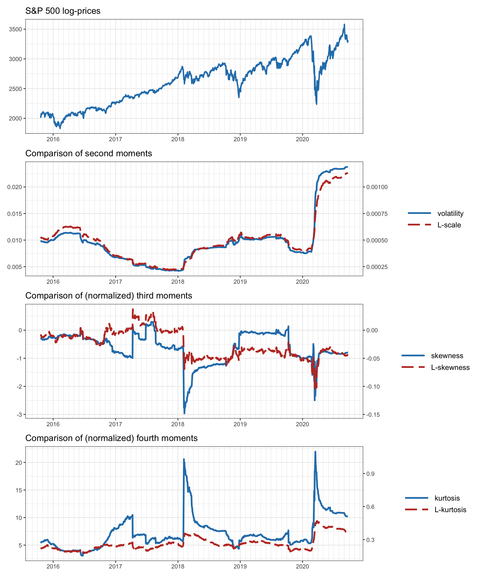
Figure 9.3: Moments and L-moments of the S&P 500 index in a rolling-window fashion.
It seems that the L-moments may be superior to the regular moments in the sense that they are more stable and convey similar useful information. However, when it comes to the portfolio design, they come with the additional difficulty of requiring sorted returns, whose ordering depends on the portfolio \(\w\): \[ \w^\T\bm{r}_1, \w^\T\bm{r}_2, \dots, \w^\T\bm{r}_T \quad\longrightarrow\quad \w^\T\bm{r}_{\tau(1)} \leq \w^\T\bm{r}_{\tau(2)} \leq \dots \leq \w^\T\bm{r}_{\tau(T)}, \] where \(\tau(\cdot)\) denotes a permutation of the \(T\) observations so that the portfolio returns are sorted in increasing order.
Thus, given the permutation \(\tau(\cdot)\), the portfolio moments can be expressed as \[\begin{equation} \begin{aligned} \hat{\phi}_1(\w) & = \frac{1}{n}\sum_{t=1}^T \w^\T\bm{r}_{\tau(t)},\\ \hat{\phi}_2(\w) & = \frac{1}{2}\frac{1}{C^T_2}\sum_{t=1}^T \left(C^{t-1}_1 - C^{T-t}_1\right) \w^\T\bm{r}_{\tau(t)},\\ \hat{\phi}_3(\w) & = \frac{1}{3}\frac{1}{C^T_3}\sum_{t=1}^T \left(C^{t-1}_2 - 2C^{t-1}_1C^{T-t}_1 + C^{T-t}_2\right) \w^\T\bm{r}_{\tau(t)},\\ \hat{\phi}_4(\w) & = \frac{1}{4}\frac{1}{C^T_4}\sum_{t=1}^T \left(C^{t-1}_3 - 3C^{t-1}_2C^{T-t}_1 + 3C^{t-1}_1C^{T-t}_2 - C^{T-t}_3\right) \w^\T\bm{r}_{\tau(t)}. \end{aligned} \tag{9.10} \end{equation}\]
References
The skewness is actually defined as the standardized or normalized third moment \(\E\left[\left((X - \bar{X})/\textm{Std}[X]\right)^3\right]\), where \(\textm{Std}[X]\) is the standard deviation of \(X\).↩︎
The kurtosis is similarly defined as the standardized or normalized fourth moment \(\E\left[\left((X - \bar{X})/\textm{Std}[X]\right)^4\right]\).↩︎
\(\textm{Gamma}(a,b)\) represents the gamma distribution of shape \(a\) and rate \(b\), which has the pdf \[f(\tau \mid a,b) = b^a \tau^{a-1} \frac{\textm{exp}(-b\tau)}{\Gamma(a)},\] where \(\Gamma(a)\) is the gamma function, \(\Gamma(a) = \int_0^\infty t^{a-1}e^{-t}\,\mathrm{d}t\).↩︎