16.2 Deep Learning
Conventional machine learning methods are limited in their ability to process raw data in the black-box model \(f(\cdot)\). For decades, constructing machine-learning systems required careful engineering and considerable domain expertise to transform the raw data into a suitable feature vector \(\bm{x}\) from which the learning subsystem could detect or classify patterns. These are known as handcrafted features, in contrast to the learned features that a deep architecture can automatically obtain, a process referred to as representation learning.
Deep learning, broadly speaking, refers to methods and architectures that can automatically learn features by means of concatenation of multiple simple – but nonlinear – modules or layers, each of which transforms the representation at one level (starting with the raw input) into a representation at a higher, slightly more abstract, level. For example, an image comes in the form of an array of pixel values, and the learned features in the first layer of representation typically represent the presence or absence of edges at particular orientations and locations in the image. The second layer typically detects motifs by spotting particular arrangements of edges. The third layer may assemble motifs into larger combinations that correspond to parts of familiar objects, and subsequent layers would detect objects as combinations of these parts. The key aspect of deep learning is that these layers of features are not designed by human engineers: they are learned from data using a general-purpose learning procedure.
Quoting LeCun et al. (2015):69
Deep learning allows computational models that are composed of multiple processing layers to learn representations of data with multiple levels of abstraction. These methods have dramatically improved the state-of-the-art in speech recognition, visual object recognition, object detection and many other domains such as drug discovery and genomics. Deep learning discovers intricate structure in large data sets by using the backpropagation algorithm to indicate how a machine should change its internal parameters that are used to compute the representation in each layer from the representation in the previous layer.
Deep learning is significantly advancing the solutions to problems that have long challenged the artificial intelligence community. In fact, deep learning has been so successful that it has been referred to with expressions such as “the unreasonable effectiveness of deep learning” and with questions like “Why does deep and cheap learning work so well?” (Lin et al., 2017).
A concise account of deep learning can be found in LeCun et al. (2015), whereas an excellent comprehensive textbook is Goodfellow et al. (2016), and a superb short online introductory book is Nielsen (2015).
16.2.1 Historical Snapshot
Some of the fundamental ingredients of neural networks take us back centuries to 1676 (the chain rule of differential calculus), 1847 (gradient descent), 1951 (stochastic gradient descent), or 1970 (the backpropagation algorithm), to name a few. A detailed historical account of deep learning can be found in Schmidhuber (2015) and Schmidhuber (2022). At the risk of oversimplifying and for illustration purposes, some pivotal historical moments in DL include:
- 1962: Rosenblatt introduces the multilayer perceptron;
- 1967: Amari suggests training multilayer perceptrons with many layers via stochastic gradient descent;
- 1970: Linnainmaa publishes what is now known as backpropagation, the famous algorithm also known as “reverse mode of automatic differentiation” (it would take four decades until it became widely accepted);
- 1974–1980: first major “AI winter” (i.e., period of reduced funding and interest in AI);
- 1987–1993: second major “AI winter”;
- 1997: LSTM networks introduced (Hochreiter and Schmidhuber, 1997);
- 1998: CNN networks established (LeCun et al., 1998);
- 2010: “AI spring” starts;
- 2012: AlexNet network achieves an error of 15.3% in the ImageNet 2012 Challenge, more than 10.8 percentage points lower than that of the runner up (Krizhevsky et al., 2012);
- 2014: GAN networks established and gained popularity for generating data;
- 2015: AlphaGo by DeepMind beats a professional Go player;
- 2016: Google Translate (originally deployed in 2006) switches to a neural machine translation engine;
- 2017: AlphaZero by DeepMind achieves superhuman level of play in the games of chess, Shogi, and Go;
- 2017: Transformer architecture is proposed based on the self-attention mechanism, which would then become the de facto architecture for most of the subsequent DL systems (Vaswani et al., 2017);
- 2018: GPT-1 (Generative Pre-Trained Transformer) for natural language processing with 117 million parameters, starting a series of advances in the so-called large language models (LLMs);
- 2019: GPT-2 with 1.5 billion parameters;
- 2020: GPT-3 with 175 billion parameters;
- 2022: ChatGPT: a popular chatbot built on GPT-3, astonished the general public, sparking numerous discussions and initiatives centered on AI safety;
- 2023: GPT-4 with ca. 1 trillion parameters (OpenAI, 2023), which allegedly already shows some sparks of artificial general intelligence (AGI) (Bubeck et al., 2023).
As of 2023, the momentum of AI systems based on deep learning is difficult to grasp and it is challenging to keep up with the state of the art. Dozens of startup companies and open-source initiatives are produced by the day, not to mention the astounding number of publications. The pace has become unimaginable and the progress impossible to forecast.
16.2.2 Perceptron and Sigmoid Neuron
The perceptron70 is a function that maps its input vector \(\bm{x}\) to a binary output value according to \[ f(\bm{x}) = \begin{cases} 1\quad \textm{if } \bm{w}^\T\bm{x} + b \geq 0,\\ 0\quad \textm{otherwise},\\ \end{cases} \] where \(\bm{w}\) is a vector of weights and \(b\) is the bias. In other words, this function is the composition of the affine function \(\bm{w}^\T\bm{x} + b\) with the nonlinear binary step function (also called the Heaviside function) \(H(z)\) defined as 1 for \(z\geq0\) and 0 otherwise, that is, \(f(\bm{x}) = H(\bm{w}^\T\bm{x} + b)\) (alternatively, with the indicator function \(I(\cdot)\), we can write \(f(\bm{x}) = I(\bm{w}^\T\bm{x} + b \geq 0)\)). The weights give different importance to the inputs and the bias is equivalent to having a nonzero activation threshold. This is a minimal approximation of how a biological neuron works.
Sigmoid neurons are similar to perceptrons, but modified so that small changes in their weights and bias cause only a small change in their output. That is the crucial fact that will allow a network of sigmoid neurons to learn. A sigmoid neuron is defined, similarly to a perceptron, as \[ f(\bm{x}) = \sigma(\bm{w}^\T\bm{x} + b), \] where \(\sigma\) is the sigmoid function defined as \(\sigma(z) = 1/(1 + e^{-z})\). Interestingly, when \(z\) is a large positive number, then \(e^{-z}\approx0\) and \(\sigma(z)\approx1\), and when \(z\) is very negative, then \(e^{-z}\rightarrow\infty\) and \(\sigma(z)\approx0\); this resembles the behavior of the perceptron.
Both the Heaviside function \(H(z)\) (also known as a step function) and the sigmoid function \(\sigma(z)\) are types of nonlinear activation functions. These nonlinearities are key components in neural networks. Otherwise, the input–output relationship would simply be linear. Figure 16.4 compares the nonlinear activation functions for the perceptron (i.e., the step function \(H(z)\)) and the sigmoid neuron (i.e., the sigmoid function \(\sigma(z)\)), as well as the popular ReLU function \(\textm{ReLU}(z) = \textm{max}(0, z)\) to be discussed later.
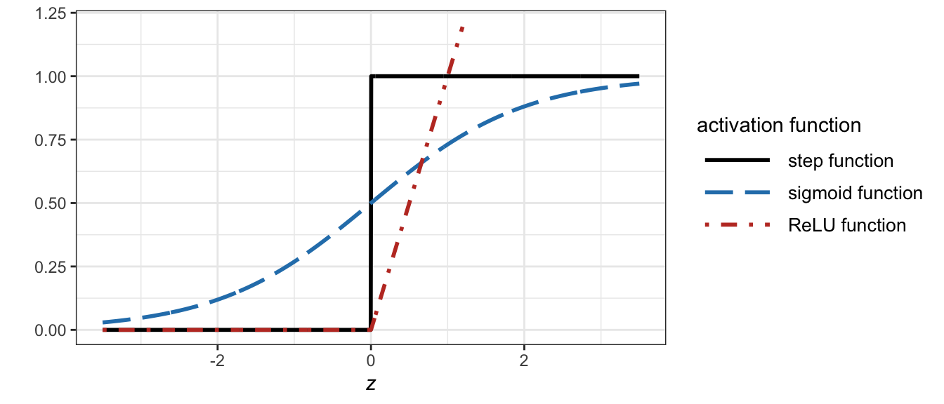
Figure 16.4: Activation functions: step function (for the perceptron), sigmoid function (for the sigmoid neuron), and ReLU (popular in neural networks).
16.2.3 Neural Networks
Perceptrons can be combined in multiple layers, leading to what is referred to as multilayer perceptron (MLP). In this way, perceptrons in subsequent layers can make decisions at a more complex and more abstract level than perceptrons in the first layer. In fact, MLPs are universal function approximators (they can approximate arbitrary functions as well as desired).
A neural network is simply several layers of neurons of any type (in fact, with some abuse of terminology they are also referred to as MLPs). The leftmost layer is called the input layer and it simply contains the input vector \(\bm{x}\) (it is not an operational layer per se). After that come the hidden layers. Finally, the rightmost layer is called the output layer and contains the output neurons. Figure 16.5 shows a four-layer network with two hidden layers.

Figure 16.5: Example of a multilayer perceptron with two hidden layers.
The goal of a neural network is to approximate some (possibly vector-valued) function \(\bm{f}\). Neural networks are often referred to as feedforward neural networks to emphasize the fact that information flows from the input \(\bm{x}\), through the intermediate layers, to the output \(\bm{y}\), without feedback connections in which outputs of the model are fed back into itself. When feedback connections are included, they are called recurrent neural networks, as presented later.
When the number of layers, called the depth of the model, is large enough, the network is referred to as deep, leading to the so-called deep neural network, as well as the mouthful of a name “deep feedforward neural network.”
Mathematically, each layer \(i\) can be thought of as implementing a vector function \(\bm{f}^{(i)}\), leading to a connected chain of functions (i.e., composition of functions), conveniently written as \[\bm{f} = \bm{f}^{(n)} \circ \dots \circ \bm{f}^{(2)} \circ \bm{f}^{(1)},\] where \(\circ\) denotes function composition. Each hidden layer of the network is typically vector valued, with their dimensionality determining the width of the model. In particular, each layer \(i\) produces an intermediate vector \(\bm{h}^{(i)}\) from the previous vector \(\bm{h}^{(i-1)}\) (with \(\bm{h}^{(0)} \triangleq \bm{x}\)) as \[ \bm{h}^{(i)} = \bm{f}^{(i)}\left(\bm{h}^{(i-1)}\right) = \bm{g}^{(i)}\left(\bm{W}^{(i)}\bm{h}^{(i-1)} + \bm{b}^{(i)}\right), \] where \(\bm{f}^{(i)}\) is the composition of an affine function with the elementwise nonlinear activation function \(\bm{g}^{(i)}.\) That is, each layer implements a function that is simply an affine function composed with a nonlinear activation function, although other operators are also used such as the max-pooling described later. Common elementwise nonlinear activation functions include:
- the sigmoid function: \[\sigma(z) = \frac{1}{1 + e^{-z}};\]
- the hyperbolic tangent: \[\textm{tanh}(z) = \frac{e^{z} - e^{-z}}{e^{z} + e^{-z}};\]
- the popular rectified linear unit (ReLU) function: \[\textm{ReLU}(z) = \textm{max}(0, z),\] which typically learns much faster in networks with many layers.
The output layer in classification problems typically employs the so-called softmax function, \[\begin{equation} \textm{softmax}(\bm{z}) = \frac{e^{\bm{z}}}{\bm{1}^\T e^{\bm{z}}}, \tag{16.1} \end{equation}\] where the exponentiation ensures the outputs are nonnegative and the normalization ensures they sum to one, that is, the output is effectively a probability mass function (in classification problems, each output value denotes the probability of each class). In regression problems, the output layer is typically a simple affine mapping without an activation function, that is, \(\bm{g}(\bm{z})=\bm{z}\).
16.2.4 Learning via Backpropagation
As mentioned earlier in Section 16.1, supervised learning involves developing a black-box model by training the system with data and minimizing an error function. This is achieved by adjusting specific parameters, commonly referred to as weights, which act as “knobs” determining the input–output function, as demonstrated in Figure 16.2. In a typical deep learning system, there may be hundreds of millions (or even billions) of these adjustable weights, and hundreds of millions of labeled examples with which to train the machine.
A conceptually simple way to learn the system is based on the gradient method. To adjust the weight vector \(\bm{w}\), the learning algorithm computes the gradient vector of the error function \(\xi(\bm{w})\), that is, \(\partial{\xi}/\partial\bm{w}\), which indicates by what amount the error would increase or decrease if the weights were increased by a tiny amount. The weight vector is then adjusted in the opposite direction to the gradient vector to minimize the error or cost function: \[ \bm{w}^{k+1} = \bm{w}^{k} - \kappa \frac{\partial{\xi}}{\partial\bm{w}}, \] where \(\kappa\) is the so-called learning rate.
The error or cost function is typically defined via a mathematical expectation over the distribution of the possible input–output pairs. In practice, it is not possible to evaluate such an expectation operator and one has to resort to a procedure called stochastic gradient descent (SGD). This process involves presenting the input vector for several examples, computing the outputs and errors, determining the average gradient for those examples, and adjusting the weights accordingly. The procedure is repeated for numerous small sets of examples from the training set until the average of the objective function ceases to decrease. It is referred to as stochastic because each small set of examples provides a noisy estimate of the average gradient across all examples. This straightforward process typically identifies a good set of weights faster in comparison to more complex optimization methods. In multilayer architectures, one can compute gradients using the backpropagation procedure, which is nothing more than a practical implementation of the chain rule for derivatives (this method was discovered independently by several different groups during the 1970s and 1980s).
In the late 1990s, neural nets and backpropagation were largely forsaken by the machine learning community and ignored by the computer vision and speech recognition communities. In particular, it was commonly thought that simple gradient descent would get trapped in poor local minima (weight configurations for which no small change would reduce the average error). In practice, however, this is rarely a problem with large networks. Regardless of the initial conditions, the system nearly always reaches solutions of very similar quality. Recent theoretical and empirical results strongly suggest that local minima are not a serious issue in general.
16.2.5 Deep Learning Architectures
Research in DL is extremely vibrant and new architectures are constantly being explored by practitioners and academics. In the following we describe some of the most relevant paradigms.
Fully-Connected Neural Networks
The neural networks previously introduced are actually fully connected neural networks in the sense that each neuron takes as inputs all the outputs from the previous layer and combines them with weights. This rapidly results in a significant increase in the number of weights to be trained as illustrated in Figure 16.6, which shows a very simple MLP with just five hidden layers.

Figure 16.6: Large number of weights in a simple multilayer perceptron with five hidden layers.
To decrease the number of weights, it is necessary to incorporate a meaningful structure into the network, tailored to the specific application being addressed. By reducing the number of weights per layer, we can have many layers to express computationally large models, producing high levels of abstraction, while keeping the number of actual parameters manageable.
Convolutional Neural Networks (CNNs)
One popular example in the history of deep learning is that of convolutional neural networks (CNNs), based on the concept of convolution commonly used in signal processing. This network achieved many practical successes during the period when neural networks were out of favor and it has been widely adopted by the computer-vision community. The origins of CNNs go back to the 1970s, but the seminal paper establishing the modern subject of convolutional networks was LeCun et al. (1998), where the architecture “LeNet-5” was proposed consisting of seven layers. Another important achievement was in 2012, with the “AlexNet” architecture (Krizhevsky et al., 2012) that blew existing image classification results out of the water.
The concept of CNNs originated from image processing, where the input is a two-dimensional image, and it makes sense for pixels to be processed only with their nearby pixels, rather than distant ones, as demonstrated in Figure 16.7. Furthermore, the weights are shifted across the image, allowing them to be shared and reused by all neurons in the hidden layer. This introduces structure in the matrix \(\bm{W}^{(i)}\) found in the affine mapping \(\bm{W}^{(i)}\bm{h}^{(i-1)} + \bm{b}^{(i)}\). Specifically, the matrix \(\bm{W}^{(i)}\) will be highly sparse (containing numerous zeros), and the nonzero elements will be repeated multiple times.

Figure 16.7: CNN filtering layer.
For instance, imagine having a \(100 \times 100\) image, which corresponds to a \(10\,000\)-dimensional input vector. If the first hidden layer has the same size (i.e., the same number of neurons), a fully connected approach would require \(10^8\) weights. In contrast, a CNN architecture would only need the coefficients of a \(5 \times 5\), that is, 25 weights plus one for the bias. Of course, we cannot really do a direct comparison between the number of parameters, since the two models are different in essential ways. But, intuitively, it seems likely that the use of translation invariance by the convolutional layer will significantly reduce the number of parameters needed to achieve performance similar to the fully-connected model. That, in turn, will result in faster training for the convolutional model and, ultimately, will help us build deep networks using convolutional layers.
To reduce network complexity, CNNs use different stride lengths (when shifting the filter) and incorporate pooling layers, such as max-pooling, after convolutional layers to condense feature maps and retain information about the presence of features without precise location details.
An interesting extension of CNNs, which are based on processing neighboring pixels, is that of graph CNNs (Scarselli et al., 2009), where the concept of neighborhood is generalized and indicated with a connectivity graph on the input elements (see Chapter 5 for details on graphs).
Recursive Neural Networks (RNNs)
Feedforward neural networks produce an output that solely depends on the current input; they do not have internal memory. Recursive neural networks (RNNs), on the other hand, are neural networks with loops in them, allowing information to persist, that is, to have memory.
Figure 16.8 depicts an RNN layer, with an internal loop that allows the implementation of a function of all previous inputs \(\bm{f}(\bm{x}_1, \bm{x}_2, \dots, \bm{x}_t)\).

Figure 16.8: RNN layer with a loop.
RNNs are appealing because they have the potential to link past information to current tasks. In instances where the gap between relevant information and its required location is small, RNNs can effectively learn to utilize past data. Nevertheless, when this gap widens significantly, standard RNNs struggle to learn how to connect the information. In theory, RNNs are fully capable of managing long-term dependencies. Yet, in practice, they often struggle to learn them due to the vanishing gradient problem during training. This issue has been addressed by introducing a specific RNN structure called LSTM.
Long Short-Term Memory (LSTM) Networks
Long short-term memory (LSTM) networks, a unique type of RNN capable of learning long-term dependencies, were introduced in Hochreiter and Schmidhuber (1997) and later refined and popularized in subsequent works. They have demonstrated remarkable success in various memory-dependent tasks, including natural language processing and time series analysis.
LSTMs are specifically engineered to tackle the long-term dependency issue. Rather than employing a basic feedback mechanism like vanilla RNNs, they utilize a complex structure composed of four interconnected sub-modules (Hochreiter and Schmidhuber, 1997), resulting in a more effective learning process compared to other RNNs.
Transformers
The transformer architecture, introduced in Vaswani et al. (2017), is a groundbreaking neural network design that revolutionized natural language processing tasks. Unlike CNNs and RNNs, transformers rely on self-attention mechanisms to process input sequences simultaneously, rather than sequentially like in RNNs. Transformers have arguably become the de facto universal architecture able to outperform existing architectures in most applications.
CNNs are adept at handling spatial data like images, while RNNs process sequential data but struggle with vanishing and exploding gradient issues. Transformers overcome these limitations by employing self-attention to weigh the importance of input elements, enabling parallel processing, faster training, and improved handling of long-range dependencies, along with position encoding to incorporate positional information.
The relevance of transformers stems from their exceptional performance on a wide range of tasks, such as machine translation, text summarization, and sentiment analysis. They form the basis of state-of-the-art models like GPT (OpenAI, 2023), which have achieved top results on benchmarks and enabled new applications, including conversational AI, automated content generation, and advanced language understanding.
Without going into the details of the architecture, it is worth a brief look at this self-attention mechanism that makes transformers unique. The idea is to present the network with all the inputs at once and let the network decide which parts of the input should influence other parts in an automatic way. Suppose that we have \(n\) inputs, each of dimension \(d\), arranged along the columns of the \(n\times d\) matrix \(\bm{V}\). The goal is to substitute each row of \(\bm{V}\) by a proper linear weighted combination of all the rows, where the weights have to be calculated so that some inputs can influence other inputs in a precise manner. The way the weights are computed in a transformer is similar to the way “keys” in a database are “queried”; that is, by using a “query” matrix \(\bm{Q}\) and a “key” matrix \(\bm{K}\) (of the same dimension as \(\bm{V}\)), we can compute the inner product of the rows of \(\bm{Q}\) and the rows of \(\bm{K}\) to get a similarity matrix \(\bm{Q}\bm{K}^\T\). At this point, we could use this similarity matrix as the weights; however, it is convenient to scale this matrix with the dimension of the keys \(\sqrt{d_k}\) and then normalize the rows so that they are nonnegative numbers with a normalized sum via the softmax operator in (16.1). Putting it all together leads to the popular expression for the so-called scaled dot-product attention (Vaswani et al., 2017), \[ \textm{Attention}(\bm{Q}, \bm{K}, \bm{V}) = \textm{softmax}\left(\frac{\bm{Q}\bm{K}^\T}{\sqrt{d_k}}\right)\bm{V}, \] which is represented in Figure 16.9. In practice, the three matrices \(\bm{Q}\), \(\bm{K}\), and \(\bm{V}\) are obtained as linear transformations of the inputs. Typically, multiple self-attention mechanisms are used in parallel.

Figure 16.9: Self-attention mechanism (scaled dot-product attention).
Autoencoder Networks
Autoencoder networks are commonly used in DL models to learn data representation via feature extraction and dimensionality reduction (Kramer, 1991). In other words, autoencoder networks perform an unsupervised feature learning process.
The architecture of an autoencoder consists, as usual, of an input layer, one or more hidden layers, and an output layer. More specifically, autoencoder networks have a symmetrical structure separated into the encoder and the decoder, with the same number of nodes in the input and output layers, and a bottleneck at the core called code or latent features, as illustrated in Figure 16.10. The network is trained so that the output is as close as possible to the input, therefore forcing the central bottleneck to condense the information, performing feature extraction in an unsupervised way.

Figure 16.10: Autoencoder structure.
Generative Adversarial Networks (GANs)
Generative adversarial networks (GANs), developed in Goodfellow et al. (2014), are a type of deep learning architecture that consists of two adversarial neural networks: a generator and a discriminator. The goal of the generator is to produce realistic data, such as images or text, while the discriminator’s role is to distinguish between real and fake data.
The generator and discriminator are trained simultaneously. During training, the generator creates synthetic data and presents it to the discriminator. The discriminator then evaluates whether the data is real or fake and provides feedback to the generator. Based on this feedback, the generator modifies its output to create more realistic data. This process continues until the generator produces data that is indistinguishable from real data, making it difficult for the discriminator to identify which data is real or fake.
GANs have been successfully used in a variety of applications, such as image generation, text-to-image synthesis, and even generating realistic music. In finance, GANs can be employed to generate artificial time series with asset prices for backtesting and stress testing purposes (Takahashi et al., 2019; Yoon et al., 2019).
Diffusion Models
Diffusion models are another type of generative model in deep learning that use a diffusion process to generate samples from a target distribution. They were first introduced in Sohl-Dickstein et al. (2015) but remained behind the curtains for a while and did not gain popularity until the 2020s (J. Ho et al., 2020; Y. Song and Ermon, 2019).
The idea is very different from the two adversarial networks (the generator and the discriminator) of GANs. Diffusion models iteratively transform an initial noise signal using a series of learnable transformations, such as neural networks, to generate samples that resemble the target distribution. At each iteration step, the model estimates the conditional distribution of the data given the current level of noise.
Both diffusion models and GANs are generative models that can be used to generate high-quality samples from complex distributions. However, diffusion models have some advantages over GANs, such as being more stable during training and not suffering from mode collapse, which is a problem where the generator produces only a small subset of the possible samples. On the other hand, GANs are more flexible and can generate a wider variety of samples, including those that are not present in the training data.
16.2.6 Applications of Deep Learning in Finance
Essentially, all the financial applications discussed in Section 16.1.5 using machine learning can also be addressed with neural networks (which are a type of ML). However, deep learning involves deep neural networks, meaning networks with many layers. With a deep architecture, there are many weights or parameters to learn, requiring a large training dataset. While abundant data in areas involving images, text, or speech is not an issue, it can be problematic in finance. Therefore, it is best to focus on financial applications with access to large datasets.
As previously described, DL has already been successfully employed in many other areas. The financial area is starting to get traction; in fact, the field is wide open and many research opportunities still exist. A comprehensive state-of-the-art snapshot (as of 2020) of the DL models developed for financial applications is provided in Ozbayoglu et al. (2020), where 144 papers are categorized according to their intended subfield in finance and also analyzed based on their DL models.
Some of the areas in finance where DL is currently being researched include financial time series forecasting, algorithmic trading (a.k.a. algo trading), risk assessment (e.g., bankruptcy prediction, credit scoring, bond rating, and mortgage risk), fraud detection (e.g., credit card fraud, money laundering, and tax evasion), portfolio management, asset pricing and derivatives markets (options, futures, forward contracts), cryptocurrency and blockchain studies, financial sentiment analysis and behavioral finance, and financial text mining (Ozbayoglu et al., 2020).
Nevertheless, the most widely studied financial application area for DL is forecasting of financial time series, particularly asset price forecasting. Even though some variations exist, the main focus is on predicting the next movement of the underlying asset. More than half of the existing implementations of DL are focused on this direction. Even though there are several subtopics of this general problem, including stock price forecasting, index prediction, forex price prediction, commodity price prediction, bond price forecasting, volatility forecasting, and cryptocurrency price forecasting, the underlying dynamics are the same in all of these applications. The majority of the DL applications for financial time series have appeared quite recently, from 2015 on, as described in the comprehensive survey (as of 2020) Sezer et al. (2020), where 140 papers are classified.
References
Yoshua Bengio, Geoffrey Hinton, and Yann LeCun (LeCun et al., 2015) were recipients of the 2018 ACM A. M. Turing Award for conceptual and engineering breakthroughs that have made deep neural networks a critical component of computing.↩︎
Perceptrons were developed in the 1950s and 1960s by the scientist Frank Rosenblatt, inspired by earlier work by Warren McCulloch and Walter Pitts.↩︎