13.3 Sparse index tracking

$ \newcommand{\bm}[1]{\boldsymbol{#1}} \newcommand{\textm}[1]{\textsf{#1}} \def\T{{\mkern-2mu\raise-1mu\mathsf{T}}} \newcommand{\R}{\mathbb{R}} % real numbers \newcommand{\E}{{\rm I\kern-.2em E}} \newcommand{\w}{\bm{w}} % bold w \newcommand{\bmu}{\bm{\mu}} % bold mu \newcommand{\bSigma}{\bm{\Sigma}} % bold mu \newcommand{\bigO}{O} %\mathcal{O} \renewcommand{\d}[1]{\operatorname{d}\!{#1}} $

The problem of sparse index tracking is in fact an instance of sparse regression and a variety of methods have been proposed in the literature to deal with the difficulty of the cardinality constraint or sparsity control (Benidis et al., 2018b, 2018a; Jansen and Van Dijk, 2002; Maringer and Oyewumi, 2007; Scozzari et al., 2013; Xu et al., 2016).

13.3.1 Tracking error

The return of an index or benchmark $r_t^\textm{b}$ is obtained from the returns of the $N$ constituent assets $\bm{r}_t \in \R^N$ via the definition of the index portfolio $\bm{b}_t > \bm{0}$ (normalized to $\bm{1}^\T\bm{b}_t = 1$) as \[\begin{equation} \bm{r}_t^\T \bm{b}_{t-1} = r_t^\textm{b},\quad t=1,\dots,T, \tag{13.3} \end{equation}\] where the vector $\bm{b}_t$ denotes the proportion of capital allocated to the assets (see Section 6.1.2 for details on notation). Note that it is also possible to define a portfolio in terms of number of shares instead of capital allocation.

If the portfolio is fixed over time, $\bm{b}_t = \bm{b}$, then the notation becomes more compact. Denoting by $\bm{X} \in \R^{T\times N}$ the matrix containing the return vectors $\bm{r}_t$ along the rows and by $\bm{r}^\textm{b} \in \R^{T}$ the vector containing the returns of the index, we can then write \[\begin{equation} \bm{X} \bm{b} = \bm{r}^\textm{b}. \tag{13.4} \end{equation}\] However, it is important to remark that in most practical cases the index portfolio changes over time and the notation in (13.3) is the correct one.

The goal is to design a sparse portfolio $\w_t$ such that $\bm{r}_t^\T \w_{t-1} \approx r_t^\textm{b}$ as in (13.3). For simplicity of notation, we can assume a fixed portfolio over time $\w_t = \w$ and then the goal can be written as the approximation $\bm{X} \w \approx \bm{r}^\textm{b}$ similarly to (13.4). Thus, probably the simplest way to define the tracking error (TE) is \[\begin{equation} \textm{TE} = \frac{1}{T}\left\|\bm{r}^\textm{b} - \bm{X}\w\right\|^2_2, \tag{13.5} \end{equation}\] which fits naturally in the context of sparse regression of Section 13.2. Further expanding this with $\bm{X} \bm{b} = \bm{r}^\textm{b}$ leads to \[ \textm{TE} = (\bm{b} - \w)^\T \frac{1}{T}\bm{X}^\T\bm{X} (\bm{b} - \w), \] which can be interpreted as an approximation of an alternative definition of the tracking error based on $\bm{b}:$ \[ \textm{TE}^\textm{b} = (\bm{b} - \w)^\T \bSigma (\bm{b} - \w), \] where $\bSigma$ is the covariance matrix of the returns. However, this requires knowledge of $\bm{b}$, which may or may not be available. In addition, in most practical cases the index portfolio $\bm{b}_t$ changes over time. Thus, the empirical error measure in (13.5) is preferred.

The tracking error definition in (13.5) is the most widely adopted measure in the literature (Benidis et al., 2018b, 2018a; Jansen and Van Dijk, 2002; Scozzari et al., 2013; Shapcott, 1992; Xu et al., 2016), with some exceptions that involve the portfolio defined in terms of number of shares (Beasley et al., 2003; Maringer and Oyewumi, 2007). Other more sophisticated measures of error are considered later in Section 13.4.

Fixed versus time-varying portfolio

The tracking error definition in (13.5) is very convenient because it fits naturally in the context of sparse regression of Section 13.2. However, it is important to remark that in most practical cases the index portfolio changes over time. For example, for cap-weighted indices (the most common ones), the normalized portfolio evolves by definition as \[ \bm{b}_t = \frac{\bm{b}_{t-1} \odot \left(\bm{1} + \bm{r}_t\right)}{\bm{b}_{t-1}^\T \left(\bm{1} + \bm{r}_t\right)}. \]

As a consequence, it makes little sense to try to approximate this time-varying portfolio $\bm{b}_t$ with a constant portfolio $\w$ (except for the convenience of the simplicity of notation). In addition, even if we really wanted a fixed portfolio $\w$, this would imply a frequent rebalancing (with the corresponding transaction cost) because the normalized portfolio would otherwise naturally change over time (see (6.1) in Chapter 6 for details) as \[ \w_t = \frac{\w_{t-1} \odot \left(\bm{1} + \bm{r}_t\right)}{\w_{t-1}^\T \left(\bm{1} + \bm{r}_t\right)}. \]

Interestingly, it is still possible to express a tracking error with more realistic time-varying portfolios in the same convenient form as (13.5). The key is the following approximation based on the assumption that the index is being tracked $\bm{r}_t^\T \w_{t-1} \approx r_t^\textm{b}$: \[ \w_t \approx \frac{\w_{t-1} \odot \left(\bm{1} + \bm{r}_t\right)}{1 + r_t^\textm{b}} \approx \w_{0} \odot \bm{\alpha}_t, \] where $\w_{0}$ is the initial portfolio and \[\begin{equation} \bm{\alpha}_t = \prod_{t'=1}^{t}\frac{\bm{1} + \bm{r}_{t'}}{1 + r_{t'}^\textm{b}} \tag{13.6} \end{equation}\] denotes weights based on the cumulative returns. This allows us to write the portfolio return as \[ \bm{r}_t^\T \w_{t-1} \approx \bm{r}_t^\T \left(\w_{0} \odot \bm{\alpha}_{t-1}\right) = \tilde{\bm{r}}_t^\T \w_{0}, \] where $\tilde{\bm{r}}_t = \bm{r}_t \odot \bm{\alpha}_{t-1}$ are properly weighted returns.

Thus, we can finally write the tracking error, similarly to (13.5), as \[\begin{equation} \textm{TE}^\textm{time-varying} = \frac{1}{T}\left\|\bm{r}^\textm{b} - \tilde{\bm{X}}\w\right\|^2_2, \tag{13.7} \end{equation}\] where now $\tilde{\bm{X}}$ contains the weighted returns $\tilde{\bm{r}}_t$ along the rows and $\w$ denotes the initial portfolio $\w_0$.

Summarizing, the formulation in (13.5) assumes a fixed portfolio (as done in most of the literature), which can be considered as a rough approximation, whereas (13.7) provides a more accurate approximation.

Figure 13.4 shows the tracking error over time with $K=20$ active assets under the approximation (or assumption) of a fixed portfolio $\w$ as in (13.5) and with the more accurate approximation of a time-varying portfolio as in (13.7), which shows improved results.

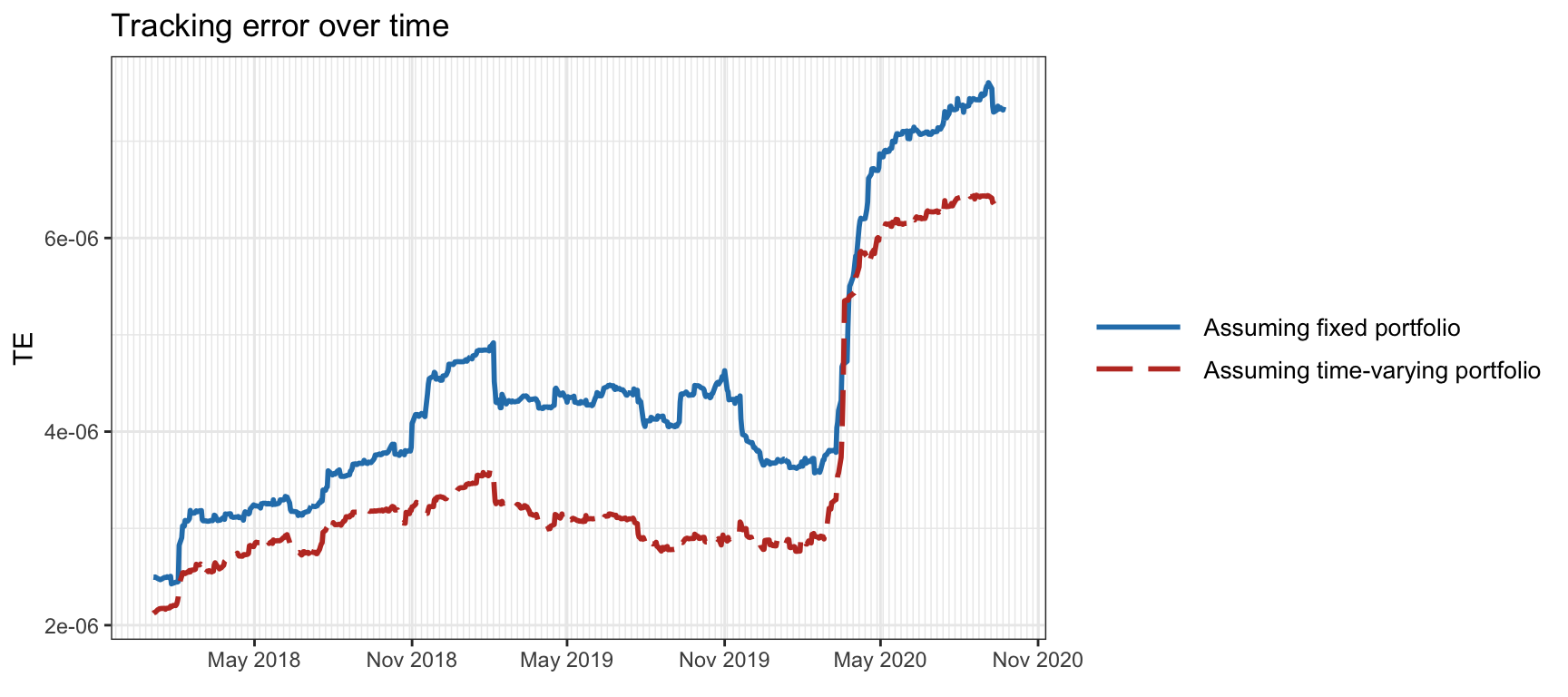
$Tracking error over time of the S\&P 500 index assuming fixed and time-varying portfolios.$

Figure 13.4: Tracking error over time of the S&P 500 index assuming fixed and time-varying portfolios.

Linear versus log-returns

Computing the portfolio returns as in (13.3)-(13.4) or, simply, using the expression $\bm{X} \w$ implicitly assumes the use of linear returns in $\bm{X}$ and $\bm{r}^\textm{b}$ (recall that linear returns are additive along assets, cf. Chapter 6).

Nevertheless, one can similarly use log-returns in $\bm{X}$ and $\bm{r}^\textm{b}$ and define the tracking error in terms of log-returns. The log-returns $\bm{r}^{\textm{log}}_t$ and the linear returns $\bm{r}^{\textm{lin}}$ are related (see Chapter 6) as \[ \bm{r}^{\textm{log}}_t = \textm{log}\left(\bm{1} + \bm{r}^{\textm{lin}}_t\right) \approx \bm{r}^{\textm{lin}}_t, \] due to the fact that $\textm{log}(1 + x) \approx x$ for small $x$. Thus, the log-returns of the portfolio $\w$ can be approximated as \[ \textm{log}\left(1 + \w^\T \bm{r}^{\textm{lin}}_t\right) \approx \w^\T \bm{r}^{\textm{log}}_t. \]

In practice, the difference between using linear or log-returns is negligible.

Plain versus cumulative returns

It is worth pointing out that minimizing the error in terms of the period-by-period returns (plain returns) does not directly imply a better track of the cumulative returns (or price) over time. The reason is that the errors in the returns can accumulate over time on a more positive or negative side. If one really wants to control the long-term deviation of the cumulative returns, then the error measure should properly reflect this, for example, by using long-term returns rather than period-by-period returns or even by using cumulative returns (Benidis et al., 2018a). However, in numerous instances, tracking an index in the short term is essential for hedging purposes against other investments. In such cases, the objective is not to outperform the index, and it is the period-by-period returns that truly matter.

The price error can be measured by the tracking error in terms of the cumulative returns as \[\begin{equation} \textm{TE}^\textm{cum} = \frac{1}{T}\left\|\bm{r}^\textm{b,cum} - \bm{X}^\textm{cum}\w\right\|^2_2, \tag{13.8} \end{equation}\] where $\bm{X}^\textm{cum}$ (similarly $\bm{r}^\textm{b,cum}$) denotes the cumulative returns, whose rows can be obtained as \[ \bm{r}^\textm{cum}_t \approx \sum_{t'=1}^{t}\bm{r}_{t'}. \] For the case of linear returns, this expression follows from the approximation \[ \prod_{t'=1}^{t}\left(\bm{1} + \bm{r}_{t'}^\T\w\right) - 1 \approx \prod_{t'=1}^{t} \textm{exp}\left(\bm{r}_{t'}^\T\w\right) - 1 = \textm{exp}\left(\sum_{t'=1}^{t}\bm{r}_{t'}^\T\w\right) - 1 \approx \left(\sum_{t'=1}^{t}\bm{r}_{t'}\right)^\T\w, \] where we have used $1 + \bm{a}^\T\w \approx \textm{exp}(\bm{a}^\T\w)$. For log-returns, it follows from \[ \textm{log}\left(\prod_{t'=1}^{t}\left(\bm{1} + \bm{r}_{t'}^\T\w\right)\right) = \sum_{t'=1}^{t} \textm{log}\left(\bm{1} + \bm{r}_{t'}^\T\w\right) \approx \left(\sum_{t'=1}^{t}\bm{r}_{t'}\right)^\T\w. \]

Figure 13.5 shows the tracking of the index price with $K=20$ active assets using plain and cumulative returns in the definition of tracking error as in (13.5) and (13.8), respectively. Clearly, the cumulative returns provide a much better tracking of the index price (although not of the tracking error in terms of returns).

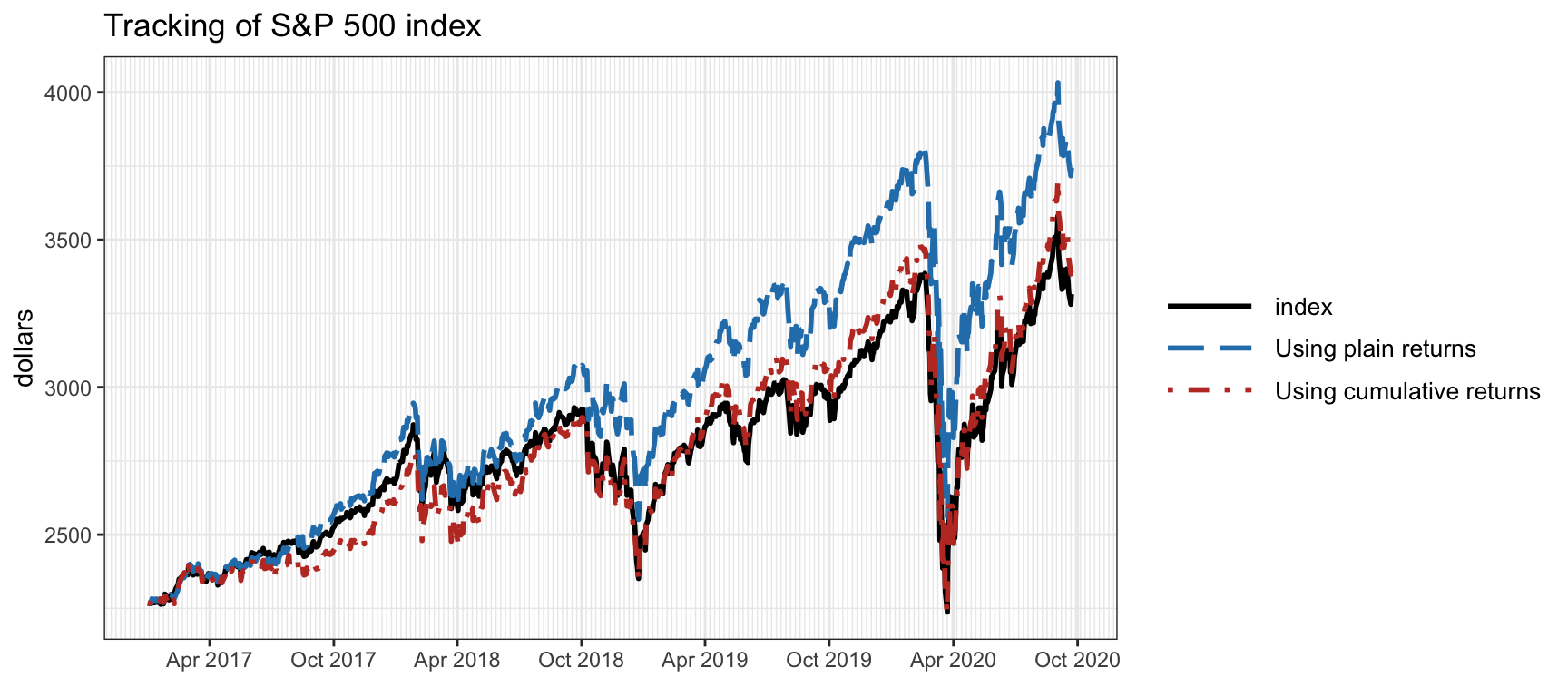
$Tracking over time of the S\&P 500 index using plain returns and cumulative returns.$

Figure 13.5: Tracking over time of the S&P 500 index using plain returns and cumulative returns.

Summary of tracking errors

Figure 13.6 summarizes the different tracking error definitions previously defined (ignoring the difference between linear and log-returns). To recall, the different data matrices employed are:

$\bm{X}$: contains the plain returns $\bm{r}_t$ along the rows;
$\tilde{\bm{X}}$: contains the weighted plain returns $\tilde{\bm{r}}_t = \bm{r}_t \odot \bm{\alpha}_{t-1}$ along the rows (with $\bm{\alpha}_t$ in (13.6));
$\bm{X}^\textm{cum}$: contains the cumulative returns $\bm{r}^\textm{cum}_t \approx \sum_{t'=1}^{t}\bm{r}_{t'}$ along the rows; and
$\tilde{\bm{X}}^\textm{cum}$: contains the weighted cumulative returns $\sum_{t'=1}^{t}\tilde{\bm{r}}_{t'}$.

Figure 13.6: Different data matrices employed in the definition of tracking error.

13.3.2 Problem formulation

Formulating the index tracking problem is quite straightforward in terms of a sparse regression problem: \[\begin{equation} \begin{array}{ll} \underset{\w}{\textm{minimize}} & \begin{aligned}[t] \frac{1}{T}\left\|\bm{r}^\textm{b} - \bm{X}\w\right\|^2_2 + \lambda \|\w\|_0 \end{aligned}\\ \textm{subject to} & \begin{aligned}[t] \w \in \mathcal{W} \end{aligned}, \end{array} \tag{13.9} \end{equation}\] where the parameter $\lambda$ controls the level of sparsity in the portfolio, $\mathcal{W}$ denotes an arbitrary constraint set, such as $\mathcal{W} = \{\w \mid \bm{1}^\T\w=1, \w\ge\bm{0} \}$, and matrix $\bm{X}$ contains the returns of the assets (any version of returns as explored in Section 13.3.1).

Index tracking is a type of passive investment that avoids the expensive transaction costs incurred by frequent trading associated with active portfolio management. Therefore, it may be advantageous to explicitly control the turnover in the formulation (13.9) by adding a penalty term or constraint to control the turnover $\| \w - \w_0 \|_1$, where $\w_0$ is the current portfolio (Benidis et al., 2018b, 2018a). In practice, other variations on the basic index tracking formulation (13.9) are commonly used and will be explored later in Section 13.4.

Recall that the cardinality operator on the portfolio $\|\w\|_0$ is noncontinuous, nondifferentiable, and nonconvex, which means that developing practical algorithms under sparsity is not trivial. We will start with some heuristic methods and build up to the state-of-the-art solutions based on MM.

13.3.3 Methods for sparse index tracking

An important observation is that if we knew a priori the active assets, then the index tracking would be a trivial convex regression problem without the difficulty of the sparsity control. This leads to the two-step approaches that first select the active assets and then proceed with the weight computation (Jansen and Van Dijk, 2002). Nevertheless, such two-step approaches are not optimal and one can always do better by solving the problem jointly in a single step. Several methods have been proposed in the literature; some of them are computationally intensive, such as mixed integer programming or differential evolution techniques (Maringer and Oyewumi, 2007), while others are computationally feasible but theoretically cannot guarantee to produce a globally optimal solution, such as the iterative reweighted $\ell_1$-norm optimization method (Benidis et al., 2018b, 2018a) or the projected gradient method (Xu et al., 2016).

Naive two-step design

This approach first selects the desired $K$ active assets from the universe of $N$ assets (with $K \ll N$) in some heuristic way (Jansen and Van Dijk, 2002). This can be done, for example, based on

the weight of the assets in the index definition (e.g., the largest $K$ assets in $\bm{b}$);
the market capitalization of the assets; or
the strength of correlation between the assets and the index.

Once the active assets have been selected, then the weights are taken directly from the index definition $\bm{b}$ if available; otherwise, one can simply do a dense regression to obtain a proxy for $\bm{b}$.

In more detail, we can define the Boolean pattern vector $\bm{s} \in \R^{N}$ based on the selected assets: \[ s_i=\begin{cases} 1\quad & \textm{if the }i\textm{-th asset is selected}\\ 0 & \textm{otherwise}, \end{cases} \]

so that $\bm{1}^\T\bm{s}=K$. Then, we can explicitly write the weights $\w$ proportional to the definition in $\bm{b}$ (although properly scaled to that $\bm{1}^\T\w=1$): \[ \w = \frac{\bm{b} \odot \bm{s}}{\bm{1}^\T(\bm{b} \odot \bm{s})}, \] where $\odot$ denotes Hadamard (elementwise) product.

Two-step design with refitted weights

This approach refines the previous one by trying to refit the weights after the selection of the active assets (Jansen and Van Dijk, 2002). To be exact, after the $K$ assets have been selected and the Boolean pattern vector $\bm{s}$ has been computed, we can form a simple regression problem over the active assets without having to deal with the sparsity issue. Thus, the original problem (13.9) becomes \[ \begin{array}{ll} \underset{\w}{\textm{minimize}} & \begin{aligned}[t] \frac{1}{T}\left\|\bm{r}^\textm{b} - \bm{X}\w\right\|^2_2 \end{aligned}\\ \textm{subject to} & \begin{aligned}[t] \w \in \mathcal{W} \end{aligned}\\ & \begin{aligned}[t] w_i = 0 \quad\textm{if}\quad s_i = 0 \end{aligned} \end{array} \] or, equivalently, \[ \begin{array}{ll} \underset{\w}{\textm{minimize}} & \begin{aligned}[t] \frac{1}{T}\left\|\bm{r}^\textm{b} - \bm{X}\w\right\|^2_2 \end{aligned}\\ \textm{subject to} & \begin{aligned}[t] \w \in \mathcal{W} \end{aligned}\\ & \begin{aligned}[t] \w \leq \bm{s}. \end{aligned} \end{array} \]

Mixed integer programming formulation

In mixed integer programming (MIP), variables are allowed to be constrained to a discrete set, making the problem nonconvex and generally with an exponential worst-case complexity. This makes this approach impractical unless the dimensionality of the problem (number of assets) is very small (Scozzari et al., 2013).

The MIP formulation of (13.9) can be written in terms of the Boolean pattern vector $\bm{s}$, which is now a variable: \[ \begin{array}{ll} \underset{\w,\bm{s}}{\textm{minimize}} & \begin{aligned}[t] \frac{1}{T}\left\|\bm{r}^\textm{b} - \bm{X}\w\right\|^2_2 \end{aligned}\\ \textm{subject to} & \begin{aligned}[t] \w \in \mathcal{W} \end{aligned}\\ & \begin{aligned}[t] \w \leq \bm{s}, \; \bm{1}^\T\bm{s}=K, \; s_i\in\{0,1\} \end{aligned}. \end{array} \]

Evolutionary algorihms

Evolutionary algorithms are a family of optimization and search techniques inspired by the process of natural evolution. They operate on populations of candidate solutions, called individuals, which evolve over time while attempting to improve their fitness. The successful solutions are selected and combined to produce new candidate solutions akin to the natural selection process in living organisms.

Evolutionary algorithms have been applied to a wide range of problems, including optimization, machine learning, and game playing. They are particularly suitable for complex, multimodal, and noisy search spaces, where traditional optimization methods might struggle. Some key advantages include their ability to explore large solution spaces, robustness against local optima, and parallelization potential.

Some popular evolutionary algorithms include genetic algorithms and differential evolution. Genetic algorithms use a binary or symbolic representation for solutions and apply genetic operators like selection, crossover, and mutation to evolve populations of chromosomes. Differential evolution focuses on continuous optimization problems and is known for its ability to tackle high-dimensional, non-linear, and noisy problems.

Evolutionary algorithms have been employed for index tracking as a way to solve the complicated nonconvex mixed-integer problem formulation. Some examples include (Shapcott, 1992), (Beasley et al., 2003), and (Maringer and Oyewumi, 2007). Nevertheless, the computational complexity of evolutionary algorithms can be high since a population of solutions have to be evolved over many generations to properly explore the nonconvex fitness surface.

Iterative reweighted $\ell_1$-norm method

Two main approaches were considered in Section 13.2 for sparse regression: based on the $\ell_1$-norm approximation and based on a concave approximation. Unfortunately, the commonly used method based on the $\ell_1$-norm $\|\w\|_1$ cannot be used in the context of portfolio optimization due to the portfolio constraints $\bm{1}^\T\w=1$ and $\w\ge\bm{0}$ that lead trivially to \[ \|\w\|_1 = \bm{1}^\T\w = 1. \]

Thus, we need to resort to a more refined concave approximation of (13.9); for example, based on the log approximation: \[\begin{equation} \begin{array}{ll} \underset{\w}{\textm{minimize}} & \begin{aligned}[t] \frac{1}{T}\left\|\bm{r}^\textm{b} - \bm{X}\w\right\|^2_2 + \lambda \sum_{i=1}^N \textm{log}\left(1 + \frac{|w_i|}{\varepsilon}\right) \end{aligned}\\ \textm{subject to} & \begin{aligned}[t] \w \in \mathcal{W} \end{aligned}. \end{array} \tag{13.10} \end{equation}\] This nonconvex problem can then be addressed with the MM framework to obtain a convenient iterative procedure called iterative reweighted $\ell_1$-norm method and summarized in Algorithm 13.1.⁵⁸

Algorithm 13.1: Iterative reweighted $\ell_1$-norm method to solve the approximated sparse index tracking problem (13.10).

Choose initial point $\w^0 \in \mathcal{W}$;
Set $k \gets 0$;
repeat

Compute weights \[\alpha_i^k = \frac{1}{\varepsilon + \left|w_i^k\right|};\]
Solve the following weighted $\ell_1$-norm problem to obtain $\w^{k+1}$: \[ \begin{array}{ll} \underset{\w}{\textm{minimize}} & \begin{aligned}[t] \frac{1}{T}\left\|\bm{r}^\textm{b} - \bm{X}\w\right\|^2_2 + \lambda \sum_{i=1}^N \alpha_i^k|w_i|\end{aligned}\\ \textm{subject to} & \begin{aligned}[t] \w \in \mathcal{W} \end{aligned}; \end{array} \]
$k \gets k+1$;

until convergence;

Since (13.10) is a nonconvex problem, the algorithm may potentially get stuck in a local minimum. In practice, for highly sparse solutions this behavior can be observed. To deal with this issue, one can start with more dense solutions, corresponding to a small value of $\lambda$, and then sequentially increase the sparsity level by increasing $\lambda$ (Benidis et al., 2018b, 2018a).

It is interesting to remark that the main step of Algorithm 13.1 requires solving an $\ell_2$-norm weighted $\ell_1$-norm problem, which can be done with a quadratic program solver (assuming the feasible set $\mathcal{W}$ only contains linear and quadratic terms). Nevertheless, it is possible in most practical cases, to further majorize the problem in order to obtain a closed-form solution without the need for a solver (Benidis et al., 2018b, 2018a).

13.3.4 Numerical experiments

Convergence of the iterative reweighted $\ell_1$-norm method

Figure 13.7 illustrates the convergence of the iterative reweighted $\ell_1$-norm method described in Algorithm 13.1. We can see that the convergence is extremely fast and that 2-3 iterations seem to reap most of the benefit.

$Convergence of the iterative reweighted $\ell_1$-norm method for sparse index tracking.$

Figure 13.7: Convergence of the iterative reweighted $\ell_1$-norm method for sparse index tracking.

Comparison of algorithms

We now compare the tracking of the S&P 500 index based on different tracking methods, namely:

the naive two-step approach with proportional weights to the index definition;
the two-step approach with refitted weights;
the iterative reweighted $\ell_1$-norm method in Algorithm 13.1; and
the MIP formulation (although the computational complexity is too high).

Figure 13.8 shows the tracking error over time of the S&P 500 index with $K=20$ active assets (the MIP method is excluded due to its huge computational cost). The tracking portfolios are computed on a rolling window basis with a lookback period of two years and recomputed every six months. To get a more complete picture, Figure 13.9 explores the trade-off of tracking error versus the number of active assets $K$ (including the MIP method). We can observe that, as expected, the joint designs are superior to the traditional two-step approaches. While the MIP formulation is impractical due to the huge computational cost, the iterative reweighted $\ell_1$-norm method exhibits a low complexity, making it a suitable approach in practice. For more exhaustive numerical comparisons, the reader is referred to (Benidis et al., 2018b, 2018a).

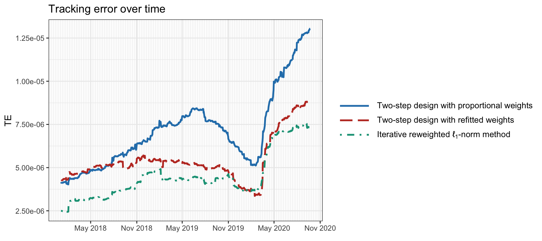
$Tracking error over time of the S\&P 500 index for different algorithms.$

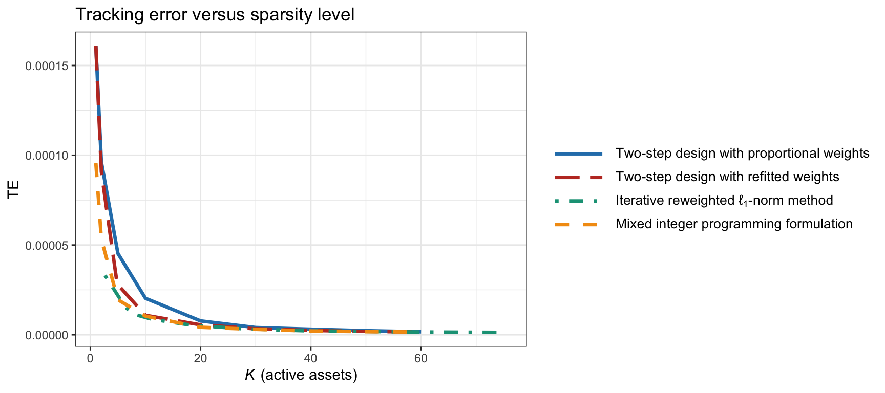
Figure 13.8: Tracking error over time of the S&P 500 index for different algorithms.

$Tracking error of the S\&P 500 index versus active assets for different algorithms.$

Figure 13.9: Tracking error of the S&P 500 index versus active assets for different algorithms.

Comparison of formulations

Finally, we consider again the comparison between assuming a fixed portfolio and a time-varying one in the definition of tracking error as in (13.5) and (13.7), respectively. This comparison was already illustrated in Figure 13.4 in terms of tracking error over time. For a more complete comparison, Figure 13.10 shows the tradeoff of tracking error versus cardinality. Indeed, the error definition in (13.7) under a time-varying portfolio is slightly more accurate.

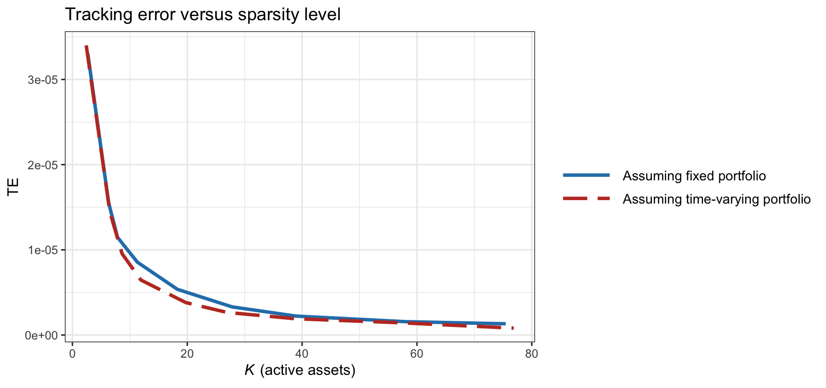
$Tracking error of the S\&P 500 index versus active assets assuming fixed and time-varying portfolios.$

Figure 13.10: Tracking error of the S&P 500 index versus active assets assuming fixed and time-varying portfolios.

References

Beasley, J. E., Meade, N., and Chang, T. J. (2003). An evolutionary heuristic for the index tracking problem. European Journal of Operational Research, 148, 621–643.

Benidis, K., Feng, Y., and Palomar, D. P. (2018a). Optimization methods for financial index tracking: From theory to practice. Foundations and Trends in Optimization, Now Publishers.

Benidis, K., Feng, Y., and Palomar, D. P. (2018b). Sparse portfolios for high-dimensional financial index tracking. IEEE Transactions on Signal Processing, 66(1), 155–170.

Benidis, K., and Palomar, D. P. (2019). sparseIndexTracking: Design of portfolio of stocks to track an index.

Jansen, R., and Van Dijk, R. (2002). Optimal benchmark tracking with small portfolios. Journal of Portfolio Management, 28(2), 33–39.

Maringer, D., and Oyewumi, O. (2007). Index tracking with constrained portfolios. Intelligent Systems in Accounting, Finance and Management, 15(1-2), 57–71.

Scozzari, A., Tardella, F., Paterlini, S., and Krink, T. (2013). Exact and heuristic approaches for the index tracking problem with UCITS constraints. Annals of Operations Research, 205(1), 235–250.

Shapcott, J. (1992). Index tracking: Genetic algorithms for investment portfolio selection. Report EPCC-SS92-24, Edinburgh Parallel Computing Centre, The University of Edinburgh.

Xu, F., Lu, Z., and Xu, Z. (2016). An efficient optimization approach for a cardinality-constrained index tracking problem. Optimization Methods and Software, 31(2), 258–271.

The R package sparseIndexTracking implements Algorithm 13.1 based on (Benidis et al., 2018b, 2018a) as well as a number of extensions covered in Section 13.4 (Benidis and Palomar, 2019). ↩︎

Portfolio Optimization