16.1 Machine Learning
The approach taken in this book has been based on first modeling the data and then designing a portfolio based on such a model, as illustrated in the big-picture diagram of Figure 1.3 in Chapter 1. In machine learning, the approach is more direct and algorithm based, attempting to learn a “black-box” model of reality (Breiman, 2001). A thorough explanation of statistical learning (which can be loosely considered equivalent to machine learning) can be found in the textbooks Hastie et al. (2009), G. James et al. (2013), and Shalev-Shwartz and Ben-David (2014).
Machine learning encompasses a variety of tools for understanding data. The fundamental paradigms of machine learning include:
Supervised learning: The task is to learn a function that maps an input to an output based on example input–output pairs (i.e., providing output labels).
Reinforcement learning: The task is again to learn a mapping function but without explicit input–output examples. Instead, it is based on a reward function that evaluates the performance of the current state and action.
Unsupervised learning: In this case, there are inputs but no supervised output (labels) or reward function. Nevertheless, one can still learn relationships and structure from such data (examples are clustering and the more sophisticated graph learning explored in Chapter 5 with applications for portfolio design in Chapter 12).
16.1.1 Black-Box Modeling
Historically, statistical learning goes back to the introduction of least squares at the beginning of the nineteenth century, what is now called linear regression. By the end of the 1970s, many more techniques for learning from data were available, but still they were almost exclusively linear methods, because fitting nonlinear relationships was computationally infeasible at the time. In the mid-1980s, classification and regression trees were introduced as one of the first practical implementations of nonlinear methods. Since that time, machine learning has emerged as a new subfield in statistics, focused on supervised and unsupervised modeling and prediction. In recent years, progress in statistical learning has been marked by the increasing availability of powerful and relatively user-friendly software.
The basic idea of ML is to model and learn the input–output relationship or mapping of some system. Denoting the input or \(p\) features as \(\bm{x}=(x_1, \dots, x_p)\) and the output as \(y\), we conjecture that reality can be modeled as the noisy relationship \[ y = f(\bm{x}) + \epsilon, \] where \(f\) is some unknown function, to be learned, that maps \(\bm{x}\) into \(y\), and \(\epsilon\) denotes the random noise. This modeling via the function \(f\) is what is usually referred to as “black box,” in the sense that no attempt is made at understanding the mapping \(f\), it is simply learned.
One of the main reasons to estimate or learn the function \(f\) is for prediction, also termed forecasting if the prediction is for a future time: assuming a given input \(\bm{x}\) is available, the output \(y\) can be predicted as \[ \hat{y} = f(\bm{x}). \]
Depending on the nature of the output \(y\), ML systems are classified into
- regression: the output is a real-valued number; and
- classification: the output can only take discrete values, such as \(\{0,1\}\) or \(\{\textm{cat},\textm{dog}\}\).
16.1.2 Measuring Performance
In order to learn the function \(f\), we need to be able to evaluate how good a candidate model is. This is conveniently done by defining an error function, also known as a loss (or cost) function. Any appropriate error function for the problem at hand can be used; the two typical choices for error functions are
- mean squared error (MSE) for regression: \[ \textm{MSE} \triangleq \E\left[\left(y - \hat{y}\right)^2\right] = \E\left[\left(y - f(\bm{x})\right)^2\right]; \]
- accuracy (ACC) for classification:68 \[ \textm{ACC} \triangleq \E\left[I\left(y = \hat{y}\right)\right] = \E\left[I\left(y = f(\bm{x})\right)\right], \] where \(I\left(y = \hat{y}\right)\) is the indicator function that equals 1 if \(y = \hat{y}\) (i.e., correct classification) and zero otherwise (i.e., classification error).
The expectation operator \(\E\left[\cdot\right]\) is over the distribution of random input–output pairs \((\bm{x},y)\). In practice, however, this expectation has to be approximated via the sample mean over some observations. To be specific, in supervised learning, the estimation or learning of the function \(f\) is performed based on \(n\) observations or data points called training data: \[\{(\bm{x}_1,y_1),(\bm{x}_2,y_2), \dots, (\bm{x}_n,y_n)\}.\] The performance or error measure can then be computed using the training data. The hope is that this training error will be close to the true error, but in practice this is not the case since the learning process can lead to a small training error that is not representative of the actual error, a phenomenon termed overfitting. To properly evaluate the performance of a system, new data that has not been used during the learning process has to be employed for testing, termed test data, producing the test performance, such as the test MSE or test ACC, which is representative of the true performance. Figure 16.1 illustrates the difference between the training MSE and the test MSE of a system as the complexity of the model \(f\) increases (i.e., the number of parameters or degrees of freedom). The divergence between the training MSE and test MSE after some point of complexity implies overfitting: the system is fitting the noise in the training data that is not representative of the test data.
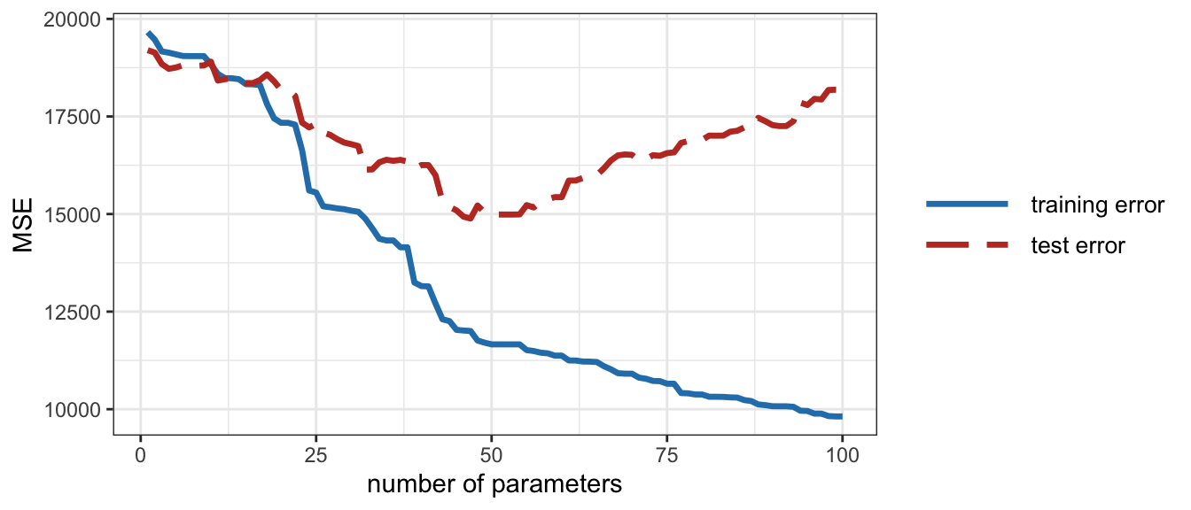
Figure 16.1: Overfitting: training error and test error.
16.1.3 Learning the Model
The black-box model \(f\) is learned based on the training data by minimizing the training error or optimizing a performance measure. The specific mechanism by which \(f\) is learned depends on the particular black-box model. For example, in artificial neural networks, the training algorithms are variations of stochastic gradient descent (described in Section 16.2).
Supervised learning is used to learn the function \(f\) based on input–output pairs (i.e., with labels) in order to minimize the error (e.g., MSE or ACC), as illustrated by the block diagram in Figure 16.2. When explicit labels are not available but the performance of the model can be measured, reinforcement learning can be effectively used, as illustrated by the block diagram in Figure 16.3.

Figure 16.2: Supervised learning in ML via error minimization.

Figure 16.3: Reinforcement learning in ML via performance optimization.
As mentioned before, extreme care has to be taken to avoid overfitting, that is, to avoid fitting the noise in the training data that is not representative of the rest of the data. In practice, this happens when there is too little training data or when the number of parameters (i.e., degrees of freedom) that characterize \(f\) is too large, as illustrated in Figure 16.1. To avoid overfitting, two main philosophies have been developed in order to choose an adequate complexity for the model (i.e., the number of degrees of freedom or parameters), termed model assessment (Hastie et al., 2009, Chapter 7):
Empirical cross-validation methods: These simply rely on assessing the performance of a learned model \(f\) (estimated from training data) on new data termed cross-validation data (note that, once the final model for \(f\) has been made, the final performance will be assessed on yet new data termed test data).
Statistical penalty methods: To avoid reserving precious data for cross-validation, these methods rely on mathematically derived penalty terms on the degrees of freedom; for example, the Bayesian information criterion (BIC), the minimum description length (MDL), and the Akaike information criterion (AIC).
16.1.4 Types of ML Models
In practice, we cannot handle a totally arbitrary function \(f\) in the whole space of possible functions. Instead, we constrain the search to some class of functions \(f\) and employ some finite-dimensional parameters, denoted by \(\bm{\theta}\), to conveniently characterize \(f\). For example, linear models correspond to the form \(f(\bm{x}) = \alpha + \bm{\beta}^\T\bm{x}\), with parameters \(\bm{\theta} = (\alpha,\bm{\beta})\). Other classes of nonlinear models can adopt more complicated structures, but always with a finite number of parameters.
Over the decades, since the advent of linear regression methods in the 1970s, a plethora of classes of functions have been proposed. The reason it was necessary to introduce so many different statistical learning approaches, rather than just a single best method, is because of the “no free lunch theorem” in statistics: no one method dominates all others over all possible data sets. On a particular data set, one specific method may work best, but some other method may work better on a different data set. Hence it is an important task to decide which method produces the best results for any given set of data. Selecting the best approach can be one of the most challenging parts of performing statistical learning in practice.
Some machine learning methods that have enjoyed success in ML include (Bishop, 2006; Hastie et al., 2009; Shalev-Shwartz and Ben-David, 2014; Vapnik, 1999):
- linear models
- sparse linear models
- decision trees
- \(k\)-nearest neighbors
- bagging
- boosting
- random forests (boosting applied to decision trees)
- support vector machines (SVM)
- neural networks, which are the foundation of deep learning.
Interestingly, some of the more complex models, such as random forests and neural networks, are so-called universal function approximators, meaning that they are capable of approximating any nonlinear smooth function to any desired accuracy, provided that enough parameters are incorporated.
16.1.5 Applications of ML in Finance
ML can be used in finance in a multitude of ways. In the context of this book, perhaps the two most obvious applications are time series forecasting and portfolio design. However, there are many other aspects where ML can be used, for example, credit risk (Atiya, 2001), sentiment analysis, outlier detection, asset pricing, bet sizing, feature importance, order market execution, big data analysis (López de Prado, 2019), and so on.
López de Prado (2018a) gives a comprehensive treatment of recent machine learning advances in finance, with extensive treatment of the preprocessing and parsing of data from its unstructured form to the appropriate form for standard ML methods to be applied. On a more practical aspect, reasons why most machine learning funds fail are presented in López de Prado (2018b).
In the realm of time series analysis, there exists a large number of publications addressing different aspects. An overview of machine learning techniques for time series forecasting is provided in Ahmed et al. (2010) and Bontempi et al. (2012), while a comparison between support vector machines and neural networks in financial time series is performed in Cao and Tay (2003). Pattern recognition in time series is covered in Esling and Agon (2012) and a comparison of various classifiers for predicting stock market price direction is provided in Ballings et al. (2015).
References
For classification systems, a large number of performance measures are commonly used, such as accuracy, precision, recall, sensitivity, specificity, miss rate, false discovery rate, among others. All these quantities are easily defined based on the number of true positives, true negatives, false positives, and false negatives. For instance, the accuracy is computed as the sum of true positives and true negatives normalized with the total number of samples.↩︎