1.1 What is Portfolio Optimization?
Suppose you observe a random variable \(X\) with mean \(\mu = \E[X]\) and variance \(\sigma^2 = \E[(X - \mu)^2]\); for example, a normal (or Gaussian) random variable \(X \sim \mathcal{N}(\mu,\sigma^2).\) The mean \(\mu\) is the value you expect to obtain, whereas the variance \(\sigma^2\) gives the variability or randomness around that value. The ratio \(\mu/\sigma\) gives a measure of the deterministic-to-random balance. In finance, \(X\) may represent the return of an investment and the ratio \(\mu/\sigma\) is called Sharpe ratio. In signal processing, it is more common to use the signal-to-noise ratio (SNR) measured in units of power and defined as \(\mu^2/\sigma^2\).
Now suppose that for each time \(t\), a different (independent) value of the random variable is observed (called a random process or random time series): \(X_t \sim \mathcal{N}(\mu,\sigma^2).\) In finance, these represent the returns of the investment, and the cumulative return is the accumulation of the previous returns, which reflects the accumulated wealth of the investment. Figure 1.1 shows a realization of such return random variables as well as the cumulative returns.
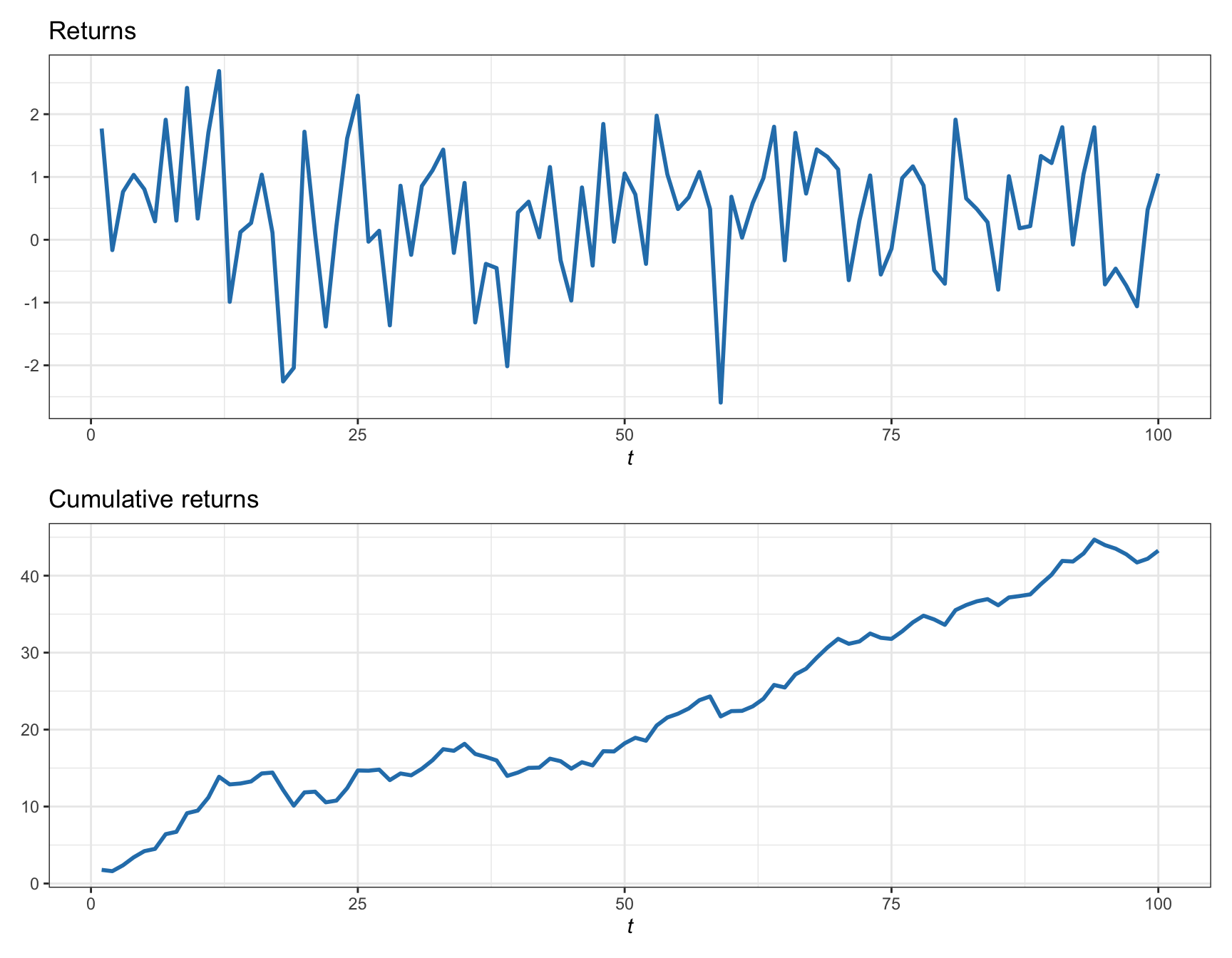
Figure 1.1: Illustration of random returns and cumulative returns.
The evolution of the cumulative returns or wealth over time, albeit random, is strongly determined by the value of the Sharpe ratio, \(\mu/\sigma\), as illustrated in Figure 1.2 for high and low values. If the Sharpe ratio is high, the cumulative return will have some fluctuations but with a consistent growth. On the other hand, if the ratio is low, the fluctuations become larger and one may even end up losing everything, leading to bankruptcy.
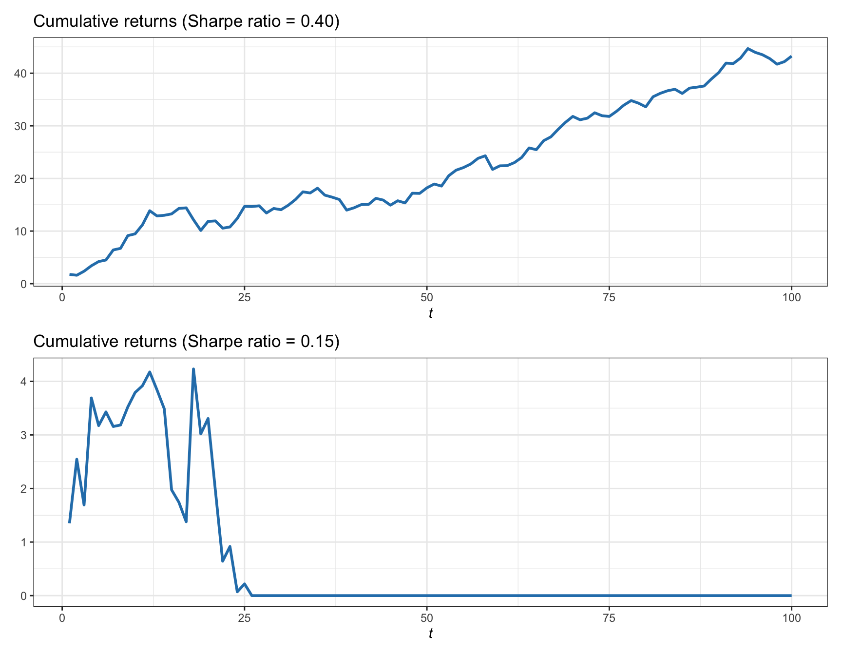
Figure 1.2: Illustration of cumulative returns with different values of Sharpe ratio.
What can an investor do to improve the cumulative return? While the random nature of the investment assets themselves cannot be changed, there are at least two dimensions that can be potentially exploited: the temporal dimension and the asset dimension.
Temporal dimension: It may be the case that the distribution of the random return \(X_t\) changes with time, leading to time-varying \(\mu_t\) and \(\sigma_t^2\). In that case, a smart investor will adapt the size of the investment to the current value of \(\mu_t/\sigma_t\). In order to do that, one needs to develop an appropriate time series model, that is, a data model at time \(t\) given the past observations. This is called data modeling and it is explored in Part I of this book.
Asset dimension: In general, an investor has a choice of \(N\) potential assets in which to invest, with returns \(X_i\) for \(i=1,\dots,N.\) Suppose they are all independent and identically distributed (i.i.d.): \(X_i \sim \mathcal{N}(\mu,\sigma^2).\) It follows from basic probability that the average of such returns, \(\frac{1}{N}\sum_{i=1}^N X_i\), preserves the mean \(\mu\) but enjoys a reduced variance of \(\sigma^2/N.\) In finance, this average is achieved by distributing the capital equally over the \(N\) assets (the popular \(1/N\) portfolio precisely implements this). In practice, however, the \(1/N\) factor in the reduction of the variance cannot be achieved because the random returns \(X_i\) are correlated among the assets, that is, the assumption of uncorrelation does not hold. Over the decades, academics and practitioners have proposed a multitude of ways to properly allocate the capital, as opposed to the baseline \(1/N\) allocation, in order to try to circumvent the inherent correlation of the assets and minimize the risk or variance. This is called portfolio optimization (also known as portfolio allocation or portfolio design) and it is covered in detail in Part II of this book.