B.6 Block Coordinate Descent (BCD)
The block coordinate descent (BCD) method, also known as the Gauss–Seidel or alternate minimization method, solves a difficult optimization problem by instead solving a sequence of simpler subproblems. We now give a brief description; for details, the reader is referred to the textbooks Bertsekas (1999), Bertsekas and Tsitsiklis (1997), and Beck (2017).
Consider the following problem where the variable \(\bm{x}\) can be partitioned into \(n\) blocks \(\bm{x} = (\bm{x}_1,\dots,\bm{x}_n)\) that are separately constrained: \[\begin{equation} \begin{array}{ll} \underset{\bm{x}}{\textm{minimize}} & f(\bm{x}_1,\dots,\bm{x}_n)\\ \textm{subject to} & \bm{x}_i \in \mathcal{X}_i, \qquad i=1,\dots,n, \end{array} \tag{B.10} \end{equation}\] where \(f\) is the (possibly nonconvex) objective function and each \(\mathcal{X}_i\) is a convex set. Instead of attempting to directly obtain a solution \(\bm{x}^\star\) (either a local or global solution), the BCD method will produce a sequence of iterates \(\bm{x}^0, \bm{x}^1, \bm{x}^2,\dots\) that will converge to \(\bm{x}^\star\). Each of these updates is generated by optimizing the problem with respect to each block \(\bm{x}_i\) in a sequential manner, which presumably will be easier to obtain (perhaps even with a closed-form solution).
More specifically, at each outer iteration \(k\), BCD will execute \(n\) inner iterations sequentially: \[ \bm{x}_i^{k+1}=\underset{\bm{x}_i\in\mathcal{X}_i}{\textm{arg min}}\;f\left(\bm{x}_1^{k+1},\dots,\bm{x}_{i-1}^{k+1},\bm{x}_i,\bm{x}_{i+1}^{k},\dots,\bm{x}_{n}^{k}\right), \qquad i=1,\dots,n. \]
It is not difficult to see that BCD enjoys monotonicity, that is, \(f\left(\bm{x}^{k+1}\right) \leq f\left(\bm{x}^k\right).\) The BCD method is summarized in Algorithm B.6.
Algorithm B.6: BCD to solve the problem in (B.10).
Choose initial point \(\bm{x}^0=\left(\bm{x}_1^0,\dots,\bm{x}_n^0\right)\in\mathcal{X}_1\times\dots\times\mathcal{X}_n\);
Set \(k \gets 0\);
repeat
- Execute \(n\) inner iterations sequentially: \[ \bm{x}_i^{k+1}=\underset{\bm{x}_i\in\mathcal{X}_i}{\textm{arg min}}\;f\left(\bm{x}_1^{k+1},\dots,\bm{x}_{i-1}^{k+1},\bm{x}_i,\bm{x}_{i+1}^{k},\dots,\bm{x}_{n}^{k}\right), \qquad i=1,\dots,n; \]
- \(k \gets k+1\);
until convergence;
B.6.1 Convergence
BCD is a very useful framework for deriving simple and practical algorithms. The convergence properties are summarized in Theorem B.3; for details, the reader is referred to Bertsekas and Tsitsiklis (1997) and Bertsekas (1999).
Theorem B.3 (Convergence of BCD) Suppose that \(f\) is (i) continuously differentiable over the convex closed set \(\mathcal{X}=\mathcal{X}_1\times\dots\times\mathcal{X}_n\), and (ii) blockwise strictly convex (i.e., in each block variable \(\bm{x}_i\)). Then every limit point of the sequence \(\{\bm{x}^k\}\) is a stationary point of the original problem.
If the convex set \(\mathcal{X}\) is compact, that is, closed and bounded, then the blockwise strict convexity can be relaxed to each block optimization having a unique solution.
Theorem B.3 can be extended by further relaxing the blockwise strictly convex condition to any of the following cases (Grippo and Sciandrone, 2000):
- the two-block case \(n=2\);
- the case where \(f\) is blockwise strictly quasi-convex with respect to \(n-2\) components; and
- the case where \(f\) is pseudo-convex.
B.6.2 Parallel Updates
One may be tempted to execute the \(n\) inner iterations in a parallel fashion (as opposed to the sequential update of BCD): \[ \bm{x}_i^{k+1}=\underset{\bm{x}_i\in\mathcal{X}_i}{\textm{arg min}}\;f\left(\bm{x}_1^{k},\dots,\bm{x}_{i-1}^{k},\bm{x}_i,\bm{x}_{i+1}^{k},\dots,\bm{x}_{n}^{k}\right), \qquad i=1,\dots,n. \]
This parallel update is called the Jacobi method. Unfortunately, even though the parallel update may be algorithmically attractive, it does not enjoy nice convergence properties. Convergence is guaranteed if the mapping defined by \(T(\bm{x}) = \bm{x} - \gamma\nabla f(\bm{x})\) is a contraction for some \(\gamma\) (Bertsekas, 1999).
B.6.3 Illustrative Examples
We now consider a few illustrative examples of applications of BCD (or the Gauss–Seidel method), along with numerical experiments.
It is convenient to start with the introduction of the popular so-called soft-thresholding operator (Zibulevsky and Elad, 2010).
Example B.5 (Soft-thresholding operator) Consider the following univariate convex optimization problem: \[ \begin{array}{ll} \underset{x}{\textm{minimize}} & \frac{1}{2}\|\bm{a}x - \bm{b}\|_2^2 + \lambda|x|, \end{array} \] with \(\lambda\geq0\).
The solution can be written as \[ x = \frac{1}{\|\bm{a}\|_2^2} \textm{sign}\left(\bm{a}^\T\bm{b}\right)\left(|\bm{a}^\T\bm{b}| - \lambda\right)^+, \] where \[ \textm{sign}(u) = \left\{\begin{array}{rl} +1 & u>0,\\ 0 & u=0,\\ -1 & u<0 \end{array}\right. \] is the sign function and \((\cdot)^+=\textm{max}(0,\cdot)\). This can be written more compactly as \[ x = \frac{1}{\|\bm{a}\|_2^2} \mathcal{S}_\lambda\left(\bm{a}^\T\bm{b}\right), \] where \(\mathcal{S}_\lambda(\cdot)\) is the so-called soft-thresholding operator defined as \[\begin{equation} \mathcal{S}_\lambda(u) = \textm{sign}(u)(|u| - \lambda)^+ \tag{B.11} \end{equation}\] and shown in Figure B.4.
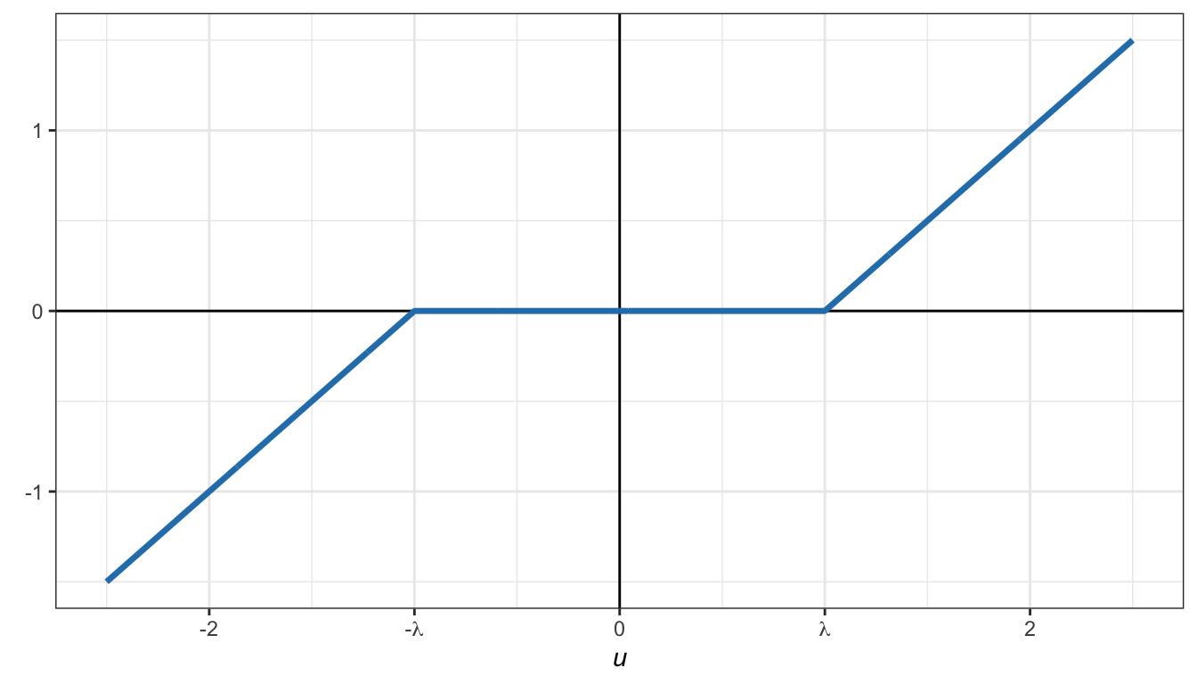
Figure B.4: Soft-thresholding operator.
One useful property of the soft-thresholding operator is the scaling property, \[ \mathcal{S}_\lambda(\kappa\times u) = \kappa\mathcal{S}_{\lambda/\kappa}(u), \] where \(\kappa>0\) is a positive scaling factor, so we can write \[ x = \frac{1}{\|\bm{a}\|_2^2} \mathcal{S}_\lambda\left(\bm{a}^\T\bm{b}\right) = \mathcal{S}_{\frac{\lambda}{\|\bm{a}\|_2^2}}\left(\frac{\bm{a}^\T\bm{b}}{\|\bm{a}\|_2^2}\right). \]
Example B.6 (\(\ell_2\)–\(\ell_1\)-norm minimization via BCD) Consider the \(\ell_2\)–\(\ell_1\)-norm minimization problem \[ \begin{array}{ll} \underset{\bm{x}}{\textm{minimize}} & \frac{1}{2}\|\bm{A}\bm{x} - \bm{b}\|_2^2 + \lambda\|\bm{x}\|_1. \end{array} \]
This problem can be easily solved with a QP solver. However, we will now derive a convenient iterative algorithm via BCD based on the soft-thresholding operator (Zibulevsky and Elad, 2010).
To be specific, we will use BCD by dividing the variable into each constituent element \(\bm{x}=(x_1,\dots,x_n)\). Therefore, the sequence of problems at each iteration \(k=0,1,2,\dots\) for each element \(i=1,\dots,n\) is \[ \begin{array}{ll} \underset{x_i}{\textm{minimize}} & \frac{1}{2}\left\|\bm{a}_ix_i - \bm{\tilde{b}}_i^k\right\|_2^2 + \lambda|x_i|, \end{array} \] where \(\bm{\tilde{b}}_i^k \triangleq \bm{b} - \sum_{j<i}\bm{a}_jx_j^{k+1} - \sum_{j>i}\bm{a}_jx_j^k.\)
This leads to the following iterative algorithm for \(k=0,1,2,\dots\): \[ x_i^{k+1} = \frac{1}{\|\bm{a}_i\|_2^2} \mathcal{S}_\lambda\left(\bm{a}_i^\T\bm{\tilde{b}}_i^k\right), \qquad i=1,\dots,n, \] where \(\mathcal{S}_{\lambda}(\cdot)\) is the soft-thresholding operator defined in (B.11). Figure B.5 shows the convergence of the BCD iterates.
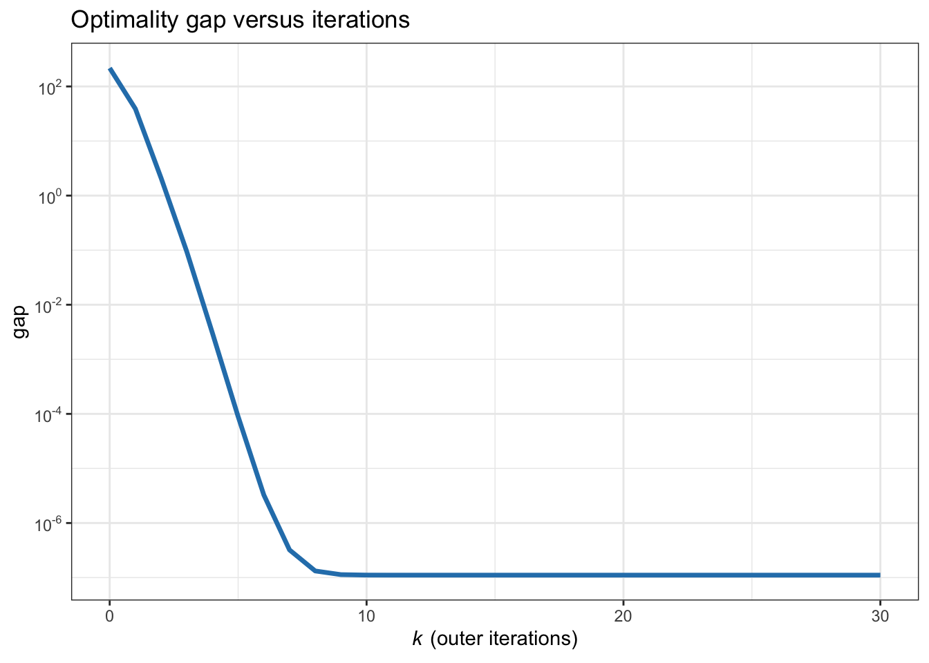
Figure B.5: Convergence of BCD for the \(\ell_2\)–\(\ell_1\)-norm minimization.