4.3 Mean Modeling
In econometrics, we are interested in forecasting the future values of a financial time series given past observations. A first choice we need to make is whether to focus on the time series of the prices or the returns. Of course they are trivially related to each other, but it is not clear a priori which one is more manageable: the returns tend to be more constant and are easier to model, whereas the prices tend to present a trend. Recall that the log-prices are denoted as \(\bm{y}_t = \textm{log}\; \bm{p}_{t}\) and the log-returns as \(\bm{x}_t = \bm{y}_t - \bm{y}_{t-1}\) (see Chapter 3 for the random walk model).
Unless otherwise stated, we will focus on the univariate case (single asset) for simplicity. In fact, in most practical cases, the multivariate case can be treated on an asset-by-asset basis. Thus, the objective is to compute the expectation of the future value of the time series at time \(t\) based on the past observations \(\mathcal{F}_{t-1}\) with the hope of extracting any structural information, that is, either \(\E[y_t \mid \mathcal{F}_{t-1}]\) for the log-prices or \(\E[x_t \mid \mathcal{F}_{t-1}]\) for the log-returns.
Readers should be aware that there might not be any significant temporal structural information to leverage. In such cases, the i.i.d. model from Chapter 3 would suffice. In fact, this is partly supported by the exploratory data analysis in Section 2.4 of Chapter 2, where the autocorrelation of the returns appears to be insignificant. Ultimately, this depends on the nature of the data and, specifically, on the frequency of the data observations.
4.3.1 Moving Average (MA)
Inspired by the i.i.d. model for the returns \(x_t = \mu + \epsilon_t\) in (3.1), the simplest way to estimate \(\mu\) is by taking the average of several observations in order to reduce the effect of the noise or innovation component \(\epsilon_t.\)
The moving average (MA) of order \(q\), denoted by MA\((q)\), is \[\begin{equation} \hat{x}_t = \frac{1}{q}\sum_{i=1}^q x_{t-i}, \tag{4.3} \end{equation}\] where \(q\) denotes the lookback and determines the amount of averaging. Since this sample mean is computed for each value of \(t\) on a rolling-window basis, it is also commonly referred to as rolling means. A noncausal variation (appropriate for smoothing but not for forecasting) considers a centered version of the moving average by using past and future samples around \(x_t\).
Observe that, under the i.i.d. model \(x_t = \mu + \epsilon_t\), the moving average is indeed estimating \(\mu\) by averaging the noise: \[ \hat{x}_t = \mu + \frac{1}{q}\sum_{i=1}^q \epsilon_{t-i}, \] where the averaged noise component has a variance reduced by a factor of \(q\). If, instead of the i.i.d. model, \(\mu_t\) is allowed to change over time, the effect of the moving average is to approximate this slowly changing value.
It is insightful to explore the interpretation of the moving average on the log-returns from the perspective of log-prices. Using \(x_t = y_t - y_{t-1}\), the moving average in (4.3) can be rewritten as \[ \hat{x}_t = \frac{1}{q} (y_{t-1} - y_{t-q-1}). \] This shows that it is effectively computing the trend of the log-prices in the form of a slope.
Alternatively, the moving average operation can be implemented on the log-prices instead of log-returns: \[\begin{equation} \hat{y}_t = \frac{1}{q}\sum_{i=1}^q y_{t-i}. \tag{4.4} \end{equation}\]
This is widely employed in the context of “charting” or “technical analysis” (Malkiel, 1973), where it is typically performed directly on the prices \(p_t\) (without the log operation). However, this does not seem to have any solid mathematical foundation apart from the visual interpretation of “smoothing” the noisy time series.
Figure 4.3 illustrates the effect of forecasting via moving averages performed on the log-prices and log-returns. As expected from the theoretical analysis, the MA on the log-prices is much worse, albeit being widely used in the “charting” community. Note that the difference of using prices instead of log-prices or using returns instead of log-returns is insignificant and not reported. Table 4.1 reports the mean squared error of the forecasting and it shows that, again, averaging the log-returns makes more sense (the lookback value \(q\) can be more carefully selected for improved performance).
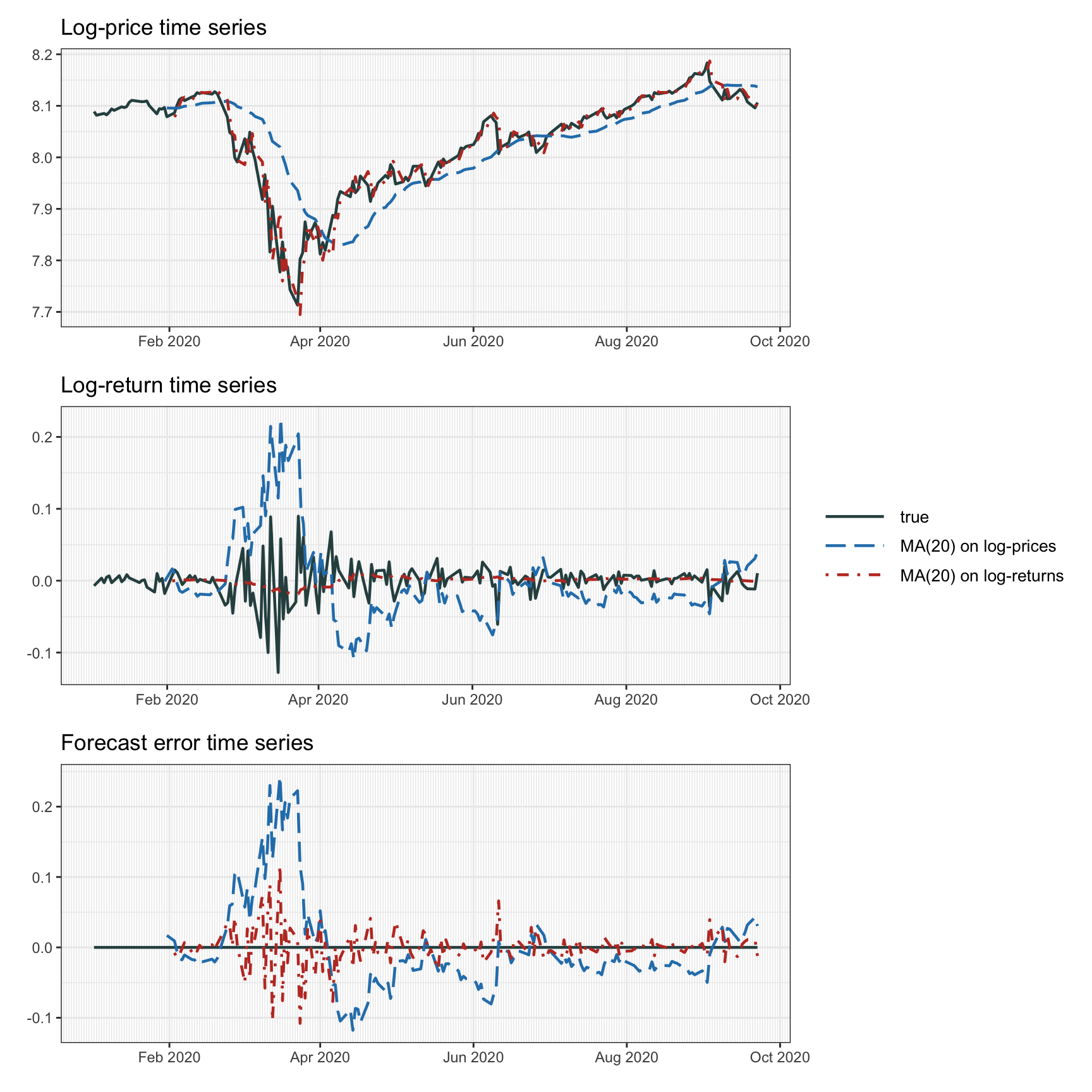
Figure 4.3: Forecasting with moving average.
| MSE | |
|---|---|
| MA(20) on log-prices | 0.004 032 |
| MA(20) on log-returns | 0.000 725 |
4.3.2 EWMA
The simple moving average in Section 4.3.1 essentially computes the average of the past observations. However, one can argue that the more recent observations should be weighted more than the less recent ones. This can be conveniently achieved with the exponentially weighted moving average (EWMA), or simply exponential moving average (EMA), with the recursive computation \[\begin{equation} \hat{x}_t = \alpha x_{t-1} + (1 - \alpha) \hat{x}_{t-1}, \tag{4.5} \end{equation}\] where \(\alpha\) (with \(0\leq\alpha\leq1\)) determines the exponential decay or memory.
We can easily see that this recursion is effectively implementing exponential weights (hence the name): \[ \hat{x}_t = \alpha x_{t-1} + \alpha(1 - \alpha) x_{t-2} + \alpha(1 - \alpha)^2 x_{t-3} + \alpha(1 - \alpha)^3 x_{t-4} + \cdots \]
4.3.3 ARMA Modeling
The “bread and butter” modeling and forecasting techniques in finance are extensions of the basic MA and EMA models previously described. These classical methods are essentially autoregressive models that attempt to capture any existing linear structure in the return time series. These models have been extensively explored for the past five decades and have reached a good level of maturity. We now summarize the basic ideas without going into any level of detail; more information can be found in the many comprehensive textbooks (Lütkepohl, 2007; Ruppert and Matteson, 2015; Tsay, 2010, 2013).
The most basic autoregressive (AR) model is of order \(1\), denoted by AR\((1)\), given as \[ x_t = \phi_0 + \phi_1 x_{t-1} + \epsilon_t, \] where \(\phi_0\) and \(\phi_1\) (as well as the variance \(\sigma^2\) of the noise term \(\epsilon_t\)) are the parameters of the model to be determined via a fitting procedure on historical data. This model attemps to capture any linear dependency between the consecutive returns. More generally, an autoregressive model of order \(p\), AR\((p)\), is given by \[ x_t = \phi_0 + \sum_{i=1}^p \phi_i x_{t-i} + \epsilon_t, \] which now contains more parameters, \(\phi_0,\dots,\phi_p\) and \(\sigma^2\), to be fitted (also, the order \(p\) has to be determined).
Similarly, we have the moving average models that attempt to exploit any linear dependency from past noise terms by averaging the last \(q\) values. Combining both components leads us to the popular autoregressive moving average (ARMA) models. In particular, an ARMA model of orders \(p\) and \(q\), denoted by ARMA\((p,q)\), is written as \[\begin{equation} x_t = \phi_0 + \sum_{i=1}^p \phi_i x_{t-i} + \epsilon_t - \sum_{j=1}^q \psi_j \epsilon_{t-j}, \tag{4.6} \end{equation}\] where now the parameters are \(\phi_0,\dots,\phi_p\), \(\psi_1,\dots,\psi_q\) and \(\sigma^2\).
Under the ARMA model in (4.6), the forecast of \(x_t\) is given by the conditional expected return \[ \hat{x}_t \triangleq \mu_t = \E[x_t \mid \mathcal{F}_{t-1}] = \phi_0 + \sum_{i=1}^p \phi_i x_{t-i}, \] with conditional variance \[ \sigma^2_t = \E[(x_t - \mu_t)^2 \mid \mathcal{F}_{t-1}] = \sigma^2, \] where \(\sigma^2\) is the (constant) variance of the noise term \(\epsilon_t\). Thus, ARMA modeling can properly deal with time-varying mean models; however, the variance is still constant. Time-varying variance models are considered in Section 4.4.
The ARMA model is defined on the log-returns \(x_t\), which are stationary (the first and second moments are time invariant), as opposed to the log-prices \(y_t\), which are nonstationary (e.g., a random walk). That is, the original log-price time series cannot be modeled directly and we have to compute the first-order difference to get \(x_t = y_t - y_{t-1}\). In general, for other types of time series, we may need to take the \(d\)th-order difference before employing an ARMA model (Tsay, 2010). This is precisely what is termed the autoregressive integrated moving average (ARIMA) model, denoted by ARIMA\((p,d,q)\), and is given by \[ x_t = \phi_0 + \sum_{i=1}^p \phi_i x_{t-i} + \epsilon_t - \sum_{j=1}^q \psi_j \epsilon_{t-j}, \] where \(x_t\) is obtained by differencing the original time series \(y_t\) \(d\) times. Thus, an ARIMA model (with \(d=1\)) on the log-prices is equivalent to an ARMA model on the log-returns.
ARMA models require the appropriate coefficients to properly fit the data. Mature and efficient software implementations are readily available in most programming languages for ARMA modeling, including the fitting process.17
All the previous models require order selection. The order of a model is characterized by the integers \(p\) and \(q\) that indicate the number of parameters. In practice, the order of a model is unknown and also has to be determined from historical data (Lütkepohl, 2007). The higher the order, the more parameters the model contains to better fit the data; however, this comes with the danger of overfitting, that is, fitting the historical data (including the noise) too well at the expense of not being able to fit the future data appropriately. The topic of overfitting is discussed in Chapter 8 in the context of backtesting. There are two main approaches to choosing the model order:
cross-validation: based on splitting the historical data into a training part and a cross-validation part, the latter being used to test the model trained with different values of orders; and
penalization methods: based on taking into account the number of parameters of the model with a penalty term in the assessment of the model, which has led to many methods, such as AIC, BIC, SIC, HQIC, and so on (Lütkepohl, 2007).
Figure 4.4 illustrates the effect of forecasting via ARMA modeling based on some specific choices of the orders, namely, i.i.d. model, AR(1), MA(1), and ARMA(1,1). Table 4.2 reports the mean squared error of the forecasts, from which we can infer that the i.i.d. modeling gives the best fit (not unexpected given the lack of strong autocorrelations in the returns).
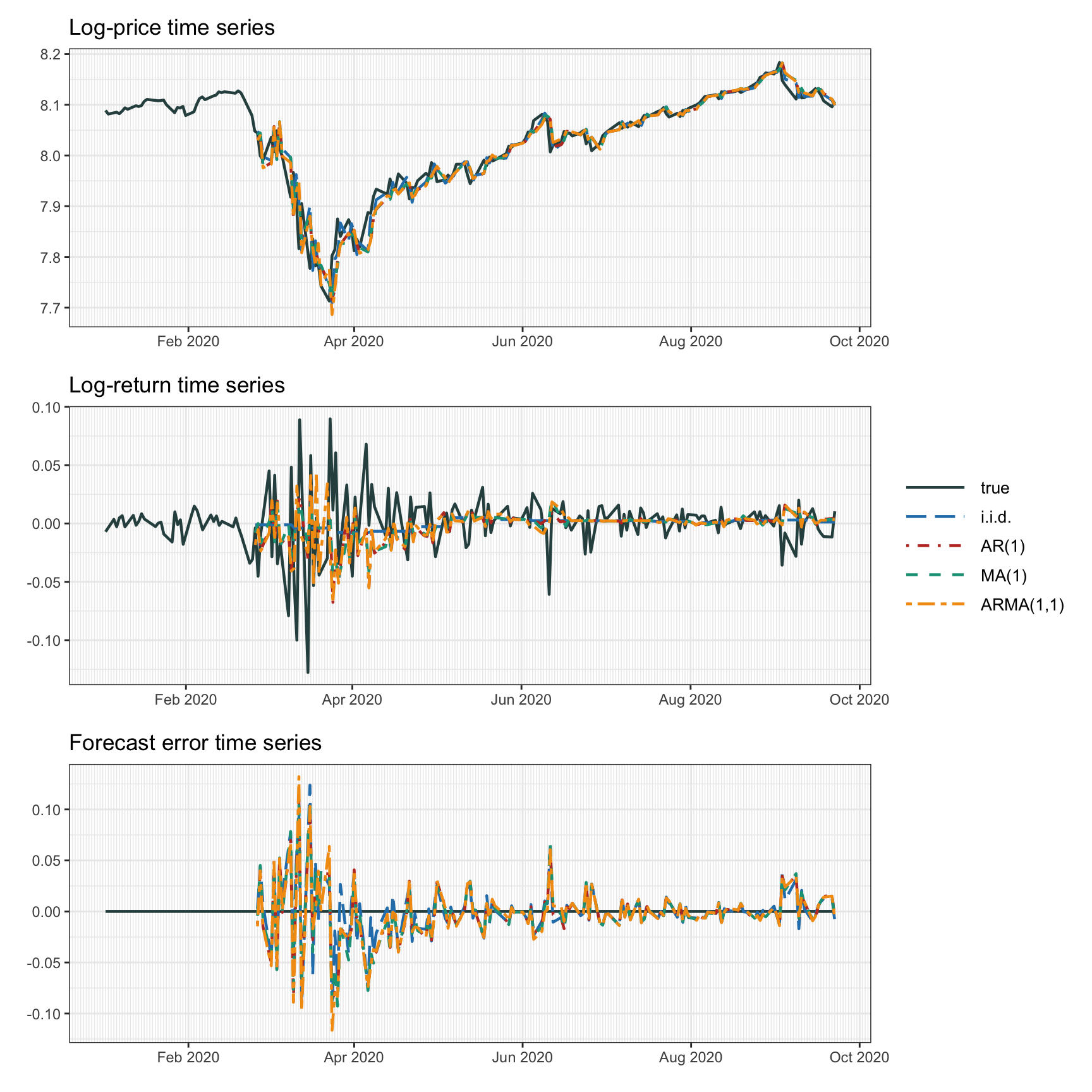
Figure 4.4: Forecasting with ARMA models.
| MSE | |
|---|---|
| i.i.d. | 0.000 754 |
| AR(1) | 0.000 793 |
| MA(1) | 0.000 805 |
| ARMA(1,1) | 0.000 914 |
4.3.4 Seasonality Decomposition
In a structural time series model, the observed time series is viewed as a sum of unobserved components such as a trend, a seasonal component, and an irregular component (Durbin and Koopman, 2012; Lütkepohl, 2007). For example, the random walk model for the log-prices, \(y_t = y_{t-1} + \mu + \epsilon_t\), can be extended to include the seasonal component \(\gamma_t\) as \[ y_t = \mu_t + \gamma_t + \epsilon_t, \] where \(\mu_t\) is the trend that can be modeled, for example, as \(\mu_t = \mu_{t-1} + \eta_t\), and the seasonal component \(\gamma_t\) (with \(s\) seasons in a period) as \(\gamma_t = -\sum_{j=1}^{s-1}\gamma_{t-j} + \omega_t\) so that the sum over a full period is approximately zero (\(\omega_t\) is a small white noise term).
The topic of time series decomposition has received a lot of attention and a wide variety of models have been proposed since the 1950s (Hyndman et al., 2008). They are often referred to as exponential smoothing methods since they are sophisticated versions of the EWMA described in Section 4.3.2 combined with the idea of decomposition of the observed time series into a variety of terms such as trend, seasonality, cycle, and so on. These methods can be extremely useful if the time series indeed contains such seasonality and cyclic components. For example, intraday financial data clearly contains specific components that change with some pattern during the day, such as the so-called “volatility smile” pattern, which refers to the volatility being higher at the beginning and end of the day, while being low during the middle of the day. Interestingly, the intraday volatility decomposition can be efficiently modeled via a state-space representation and implemented with the Kalman algorithm (R. Chen et al., 2016; Xiu and Palomar, 2023).
4.3.5 Kalman Modeling
The random walk model for the log-prices, \(y_t = y_{t-1} + \mu + \epsilon_t\) with \(\epsilon_t \sim \mathcal{N}(0, \sigma^2)\), is equivalent to the i.i.d. model for the log-returns, \(x_t = \mu + \epsilon_t\), and the results of Chapter 3 can be used to fit the time series. Realistically, the drift parameter \(\mu\) (as well as the volatility \(\sigma^2\)) will surely be time-varying. The state-space model (4.2) and the Kalman algorithm, described in Section 4.2, can be effectively used precisely to allow some time variation on the drift by treating it as a hidden state that evolves over time. In addition, it allows a more precise separation of the noise into observational noise and drift noise as described next.
The simple moving average used in (4.3) on the log-returns follows naturally from the i.i.d. model \(x_t = \mu + \epsilon_t\) as a way to estimate \(\mu\). That is, we can reinterpret (4.3) in terms of estimating the drift \(\mu\) based on the historical data up to time \(t-1\), \[ \hat{\mu}_t = \frac{1}{m}\sum_{i=1}^m x_{t-i}, \] and then forecasting the value at time \(t\) as \(\hat{x}_t = \hat{\mu}_t\). Instead, we can conveniently use a state-space model to allow the drift to slowly change over time by modeling the drift as the hidden state, \(\alpha_t = \mu_t\), that evolves over time. This is the so-called local level model (Durbin and Koopman, 2012): \[\begin{equation} \begin{aligned} x_t &= \mu_t + \epsilon_t\\ \mu_{t+1} &= \mu_t + \eta_t, \end{aligned} \tag{4.7} \end{equation}\] where the noise term \(\eta_t\) allows \(\mu_t\) to evolve over time. This model is expected to be more accurate than the simple moving average in (4.3). In addition, there is no parameter \(q\) to be chosen like in the MA\((q)\) in (4.3). Of course, this model still requires the values of the variances of the noise terms, which can be chosen a priori or learned automatically via maximum likelihood.
Alternatively, the moving average was used in (4.4) on the log-prices in a rather heuristic way to smooth the otherwise noisy time series. We can again use a state-space model to improve the modeling. For example, if we define the hidden state \(\alpha_t\) as a noiseless version of the log-prices, \(\alpha_t = \tilde{y}_t\), we can write \[\begin{equation} \begin{aligned} y_t &= \tilde{y}_t + \epsilon_t,\\ \tilde{y}_{t+1} &= \tilde{y}_t + \mu + \eta_t, \end{aligned} \tag{4.8} \end{equation}\] which allows for some observation noise via \(\epsilon_t\) and some noise in the state transition via \(\eta_t\). We can also allow the drift to be time-varying, \(\mu_t\), by augmenting the hidden state as \(\bm{\alpha}_t = \begin{bmatrix} \tilde{y}_t\\ \mu_t \end{bmatrix}\), leading to the so-called local linear trend model (Durbin and Koopman, 2012): \[\begin{equation} \begin{aligned} y_t &= \begin{bmatrix} 1 & 0 \end{bmatrix} \begin{bmatrix} \tilde{y}_t\\ \mu_t \end{bmatrix} + \epsilon_t,\\ \begin{bmatrix} \tilde{y}_{t+1}\\ \mu_{t+1} \end{bmatrix} &= \begin{bmatrix} 1 & 1\\ 0 & 1 \end{bmatrix} \begin{bmatrix} \tilde{y}_t\\ \mu_t \end{bmatrix} + \bm{\eta}_t. \end{aligned} \tag{4.9} \end{equation}\]
Figure 4.5 illustrates the effect of forecasting via Kalman filtering based on the previous three models, namely, Kalman on log-returns (with dynamic drift \(\mu_t\)), Kalman on log-prices (with static drift \(\mu\)), and Kalman on log-prices (with dynamic drift \(\mu_t\)). The difference is small. Table 4.3 reports the mean squared error of the forecasts, from which we can appreciate that as the models become more accurate the performance improves. Nevertheless, from a practical standpoint, one has to make a decision of complexity vs. meaningful performance. As a final remark, note that the performance of Kalman modeling is better than the previously explored models, namely, MA, EWMA, and ARMA.
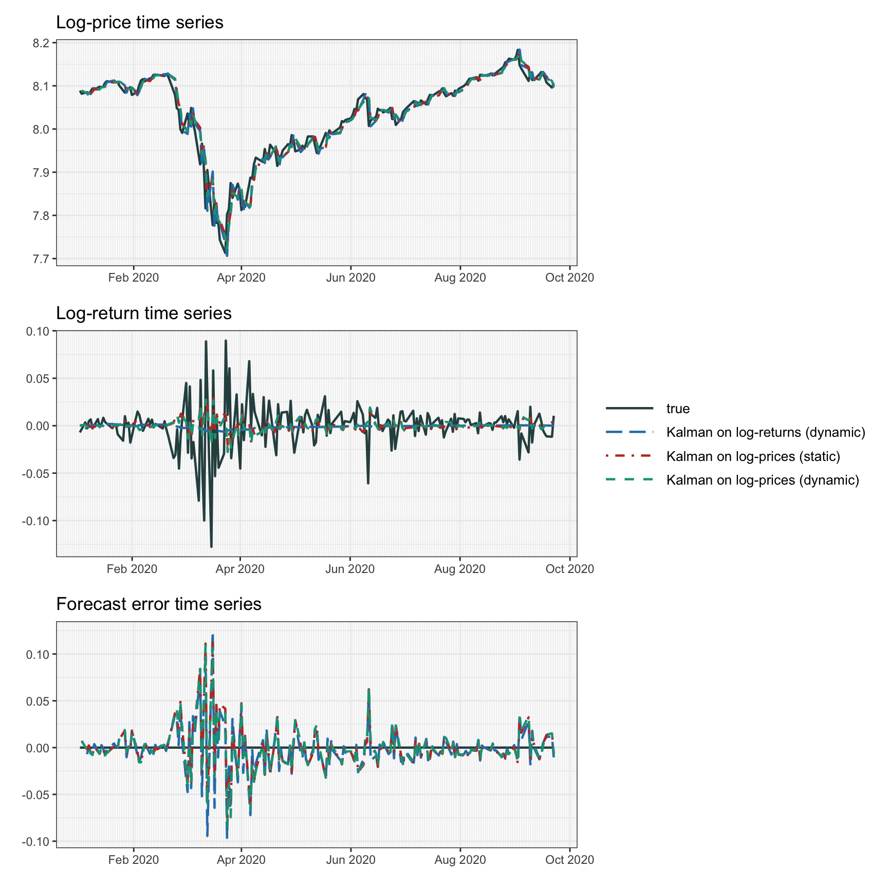
Figure 4.5: Forecasting with Kalman.
| MSE | |
|---|---|
| Kalman on log-returns (dynamic) | 0.000 632 |
| Kalman on log-prices (static) | 0.000 560 |
| Kalman on log-prices (dynamic) | 0.000 557 |
It is worth mentioning that Kalman filtering can be employed in the context of ARMA modeling from Section 4.3.3 simply by rewriting the ARMA model in (4.6), \(x_t = \phi_0 + \sum_{i=1}^p \phi_i x_{t-i} + \epsilon_t - \sum_{j=1}^q \psi_j \epsilon_{t-j}\), in terms of the state-space model in (4.2). This can be done in a multitude of ways (Durbin and Koopman, 2012; Lütkepohl, 2007; Tsay, 2010; Zivot et al., 2004). For example, an AR\((p)\) can be modeled by defining the hidden state as \(\bm{\alpha}_t = \begin{bmatrix} x_t\\ \vdots\\ x_{t-p+1} \end{bmatrix}\), leading to \[ \begin{aligned} x_t &= \begin{bmatrix} 1 & 0 & \dots & 0 \end{bmatrix} \bm{\alpha}_t,\\ \bm{\alpha}_{t+1} &= \begin{bmatrix} \phi_0\\ 0\\ \vdots\\ 0 \end{bmatrix} + \begin{bmatrix} \phi_1 & \dots & \phi_{p-1} & \phi_p\\ 1 & \dots & 0 & 0\\ \vdots & \ddots & \vdots & \vdots\\ 0 & \dots & 1 & 0\\ \end{bmatrix} \bm{\alpha}_t + \begin{bmatrix} \epsilon_t\\ 0\\ \vdots\\ 0 \end{bmatrix}. \end{aligned} \]
4.3.6 Extension to the Multivariate Case
In practice, we typically deal with \(N\) assets, so the previous univariate mean modeling approaches need to be extended to the multivariate case, which is quite straightforward. In fact, the simple MA and EWMA models from Sections 4.3.1 and 4.3.2 can be directly applied to each of the assets separately. We will next briefly describe the extension for ARMA modeling and for the state-space representation of Kalman modeling.
VARMA
The ARMA model in Section 4.3.3 can be straightforwardly extended to the multivariate case by using matrix coefficients instead of scalar coefficients. Similarly to the ARMA\((p,q)\) model in (4.6), a vector ARMA (VARMA) model of orders \(p\) and \(q\), denoted by VARMA\((p,q)\), becomes \[\begin{equation} \bm{x}_t = \bm{\phi}_0 + \sum_{i=1}^p \bm{\Phi}_i \bm{x}_{t-i} + \bm{\epsilon}_t - \sum_{j=1}^q \bm{\Psi}_j \bm{\epsilon}_{t-j}, \tag{4.10} \end{equation}\] where now the parameters are \(\bm{\phi}_0 \in \R^N\), \(\bm{\Phi}_1,\dots,\bm{\Phi}_p\in\R^{N\times N}\), \(\bm{\Psi}_1,\dots,\bm{\Psi}_q\in\R^{N\times N}\), and \(\bm{\Sigma}\in\R^{N\times N}\) is the covariance matrix of \(\bm{\epsilon}_t\).
While this extension looks trivial on paper, it quickly becomes impractical due to the exploding number of parameters. For the ARMA\((p,q)\) model in (4.6) the number of parameters is simply \(1+p+q+1\), whereas in the VARMA\((p,q)\) case it increases to \(N + (p+q)\times N^2 + N(N-1)/2\), which grows as \(N^2\). In other words, the number of parameters quickly explodes quadratically with the number of assets. The danger of fitting a model with such a large number of parameters is overfitting. This can be mitigated by either having a large number of observations in the historical data (which is rarely the case in financial applications) or by reducing the number of parameters, for example by forcing the matrix coefficients to be sparse. Note that if the matrix coefficients are forced to be diagonal matrices, then the model trivially reduces to asset-by-asset ARMA modeling.
VECM
Interestingly, in the multivariate case, a new model emerges based on the concept of cointegration, termed the vector error correction model (VECM) (Engle and Granger, 1987). The VECM model was proposed as a way to apply the ARMA model on the log-prices instead on the log-returns as in Section 4.3.3. The danger of modeling directly the log-prices is the lack of stationarity, which is why the safe approach is to differentiate first to obtain the log-returns prior to any modeling. However, the process of differentiating may potentially destroy some structure in the time series. Applying a VAR\((p)\) model on the log-prices \(\bm{y}_t\) and using \(\bm{x}_t = \bm{y}_t - \bm{y}_{t-1}\), the model can be finally written in terms of the log-returns as \[ \bm{x}_t = \bm{\phi}_0 + \bm{\Pi}\bm{y}_{t-1} + \sum_{i=1}^{p-1} \tilde{\bm{\Phi}}_i \bm{x}_{t-i} + \bm{\epsilon}_t, \] where the matrix coefficients \(\tilde{\bm{\Phi}}_i\) can be straightforwardly related to \(\bm{\Phi}_i\) in (4.10) (Tsay, 2013).
Even though this model is written in terms of the log-returns \(\bm{x}_t\), there is a new term that contains the log-prices: \(\bm{\Pi}\bm{y}_{t-1}\). As it turns out, the matrix \(\bm{\Pi}\) is of utmost importance: by decomposing it as \(\bm{\Pi}=\bm{\alpha}\bm{\beta}^\T\), the matrix \(\bm{\beta} \in \R^{N\times r}\), with \(r\) being the number of columns, reveals that the nonstationary log-prices \(\bm{y}_t\) become stationary after multiplication with \(\bm{\beta}^\T\), that is, they are cointegrated. This cointegration relationship is key in the design of mean-reverting time series in the context of pairs trading or statistical arbitrage considered in Chapter 15.
Multivariate Kalman Modeling
Finally, we can consider a state-space model for Kalman filtering, as in Section 4.3.5, properly extended to the vector case. For simplicity, we focus on the local trend model in (4.7). If we apply it on an asset-by-asset basis for \(i=1,\dots,N\), we simply obtain \[ \begin{aligned} x_{i,t} &= \mu_{i,t} + \epsilon_{i,t},\\ \mu_{i,t+1} &= \mu_{i,t} + \eta_{i,t}, \end{aligned} \] where \(\epsilon_{i,t} \sim \mathcal{N}(0, h_i)\) is the observation noise and \(\eta_{i,t} \sim \mathcal{N}(0, q_i)\) is the drift noise. However, if we allow the noise terms for the different assets to be correlated, then we can write the more general vector model \[ \begin{aligned} \bm{x}_{t} &= \bm{\mu}_{t} + \bm{\epsilon}_{t},\\ \bm{\mu}_{t+1} &= \bm{\mu}_{t} + \bm{\eta}_{t}, \end{aligned} \] where now the observation noise vector is \(\bm{\epsilon}_{t} \sim \mathcal{N}(0, \bm{H})\) and the drift noise vector is \(\bm{\eta}_{i,t} \sim \mathcal{N}(0, \bm{Q})\), both of which can model the asset correlation.
References
The R package
rugarchimplements algorithms for fitting a wide range of different ARMA models to time series data (Ghalanos, 2022). Many other packages are also available in R. The Python packagestatsmodelscontains a number of statistical data modeling methods. ↩︎