6.3 Performance Measures
There are many ways to assess the performance of a portfolio. The key quantity in most of the performance measures is the portfolio return over time (6.4), which for the case of a fixed portfolio \(\w\) can be written as in (6.8): \(R^\textm{portf}_t = \w^\T\bm{r}_t\) (for the sake of notation we use \(\bm{r}_t\) to denote the linear returns \(\bm{r}^{\textm{lin}}_t\)). We now list the most commonly used performance measures; for a detailed and extensive treatment, see Bacon (2008).
6.3.1 Expected Return
The expected return of the portfolio is simply given by \[\E\left[R_t^\textm{portf}\right] = \w^\T\bmu,\] which is actually the expected return over one period \(t\). This measure quantifies the average benefit of the investment but ignores the risk.
In most cases, however, it is the annualized return that is reported. This simply requires scaling with a factor equal to the number of periods over a year, \(\gamma\), leading to \[\textm{Annualized Return} = \gamma\times\w^\T\bmu.\]
Suppose the periods are days (i.e., daily prices); if we trade on the stock market then \(\gamma=252\) is typically the number of tradable days per year (excluding weekends and holidays, which depend on the country), whereas on cryptocurrency markets \(\gamma=365\) since they operate nonstop. Suppose now that the periods are hours (i.e., hourly prices); then the scaling factor in cryptocurrency markets would be \(\gamma=365\times24=8760\) (in stock markets it really depends on the country, since the hours per day differ and range from 5 to 9).
Given a sequence of \(T\) portfolio returns, the annualized return can be computed via the sample mean, \[ \frac{\gamma}{T}\sum_{t=1}^T R_t^\textm{portf}, \] which implicitly assumes the use of arithmetic chaining to aggregate the returns. If, instead, one uses a geometric chaining to take into account compounding, the geometric mean should be used: \[ \left(\prod_{t=1}^T \left(1 + R_t^\textm{portf}\right)\right)^{\gamma/T} - 1, \] which is also termed compound annual growth rate (CAGR). Note that the geometric mean is always smaller than the arithmetic mean (i.e., with \(\gamma=1\)); however, once the annualization with the factor \(\gamma\) is included, nothing can be said anymore. For example, an arbitrary sequence of returns has arithmetic mean 0.0047 and geometric mean 0.0040, but after annualizing with \(\gamma=100\) they become 0.47 and 0.49, respectively.
6.3.2 Volatility
The volatility is the standard deviation of the portfolio return: \[\textm{Std}\left[R_t^\textm{portf}\right] = \sqrt{\w^\T\bSigma\w}.\] It is the simplest measure of risk of a portfolio. For convenience, one may also use the square of the volatility, that is, the variance of the portfolio return, as used by Markowitz in his seminal paper (Markowitz, 1952).
To obtain the annualized volatility we need to multiply by the square root of the number of periods per year \(\gamma\): \[\textm{Annualized Volatility} = \sqrt{\gamma}\times\sqrt{\w^\T\bSigma\w}.\]
6.3.3 Volatility-Adjusted Returns
Comparing portfolios by looking at the cumulative returns may be misleading since each portfolio may have a different volatility, since it is expected that a higher-volatility portfolio will also have a higher cumulative return (assuming a bull market). To get rid of this volatility artifact when comparing portfolios, some practitioners prefer to use the volatility-adjusted returns defined as \[ \bar{R}^\textm{portf}_t = \w^\T\bm{r}_t \times \frac{\sigma^\textm{target}}{\sigma_t}, \] where \(\sigma_t\) denotes the volatility of \(\w^\T\bm{r}_t\) and \(\sigma^\textm{target}\) is the desired target volatility for the portfolio.
Figure 6.8 compares the cumulative returns of two stocks (AMD and AMZN) with and without volatility adjustment. One can observe how from the non-adjusted version AMD may look better than AMZN, but this is misleading because it comes with much higher volatility. From the volatility-adjusted version, instead, it seems that AMZN has a better trade-off of final return and volatility. In fact, this trade-off is precisely captured by the Sharpe ratio described next.
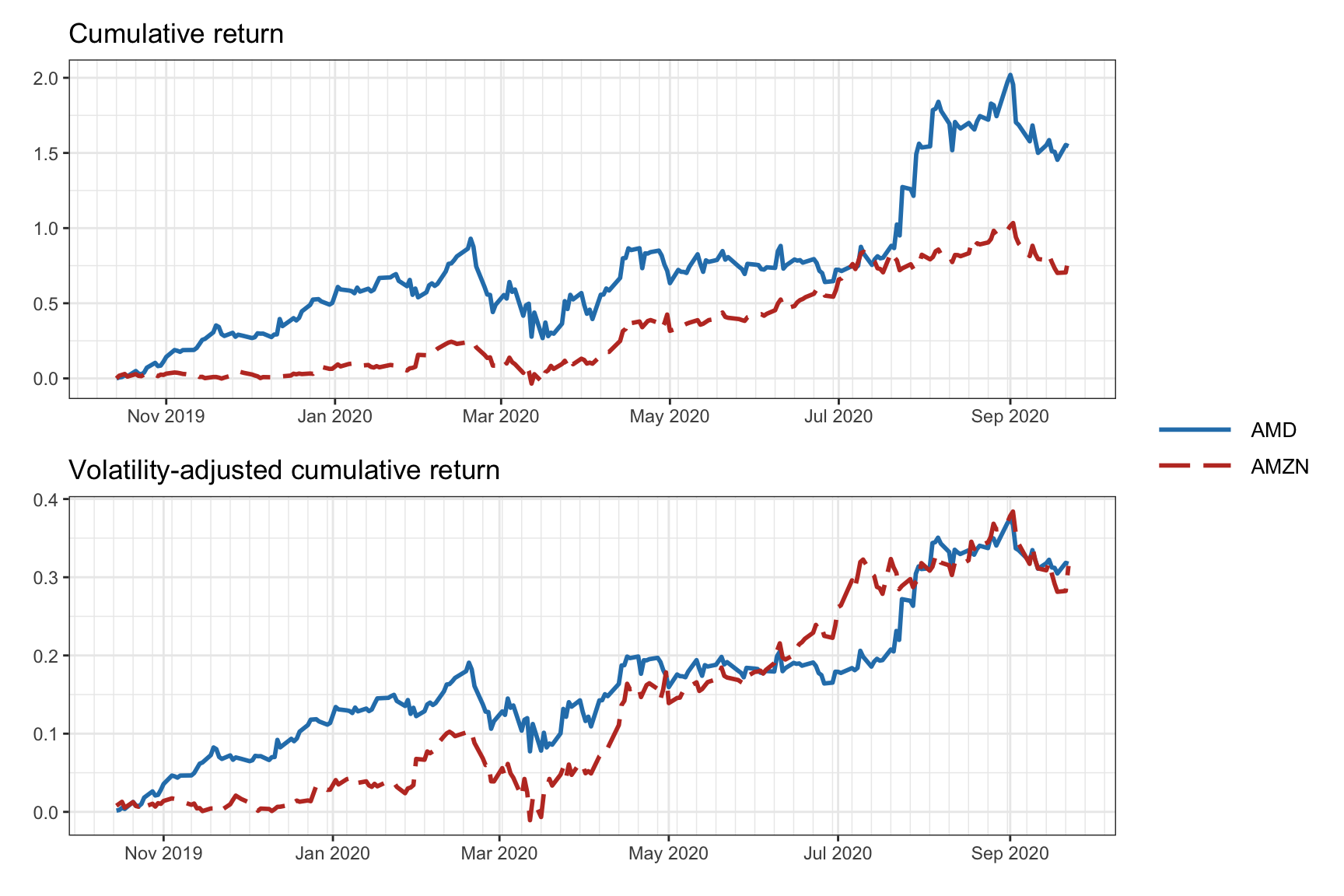
Figure 6.8: Cumulative returns and volatility-adjusted cumulative returns.
6.3.4 Sharpe Ratio (SR)
The Sharpe ratio (SR) is the risk-adjusted expected excess return, \[\textm{SR} = \frac{\w^\T\bmu - r_\textm{f}}{\sqrt{\w^\T\bSigma\w}},\] where \(r_\textm{f}\) is the risk-free rate (e.g., the interest rate on a three-month U.S. Treasury bill). It was proposed by William Sharpe in 1966 (Sharpe, 1966); see also Sharpe (1994).
Observe that the numerator is the excess return with respect to the risk-free rate; in practice, one may assume \(r_\textm{f}\approx0\) and just use the expected return. Dividing by the risk gives the risk-adjusted return, that is, the return per unit of risk.
The annualized SR is \[\textm{Annualized SR} = \sqrt{\gamma}\times\frac{\w^\T\bmu - r_\textm{f}}{\sqrt{\w^\T\bSigma\w}},\] where \(\gamma\) denotes the number of periods over a year as introduced in Section 6.3.1.
For long periods of time, rather than simply computing the overall SR, it may be useful to compute the rolling SR, which is the time series of the SR over time computed on a rolling-window basis. Figure 6.9 shows the cumulative return and rolling annualized Sharpe ratio (with a rolling window of one month) of the \(1/N\) portfolio with average Sharpe ratio of 1.65 over a universe of five stocks.
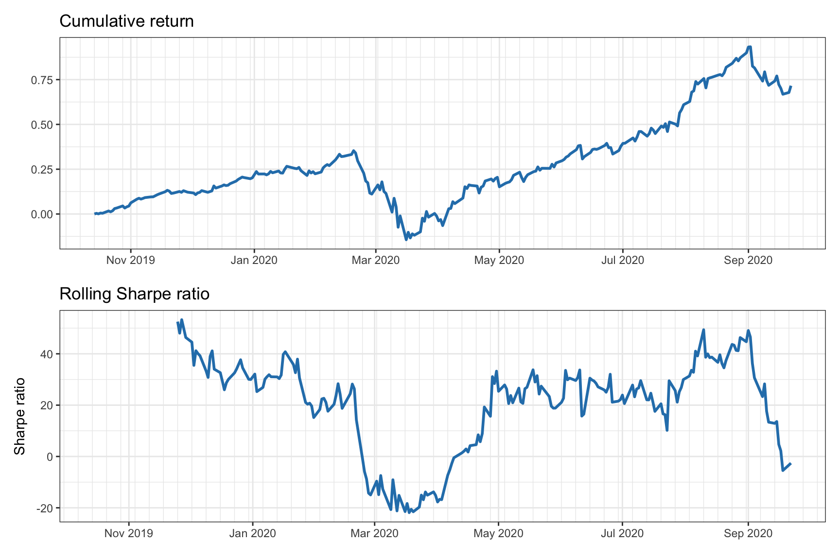
Figure 6.9: Cumulative returns and rolling annualized Sharpe ratio.
Finally, it is worth mentioning that it is common among practitioners to use the compounded annualized return in the numerator of the Sharpe ratio (i.e., using the geometric mean as previously mentioned in Section 6.3.1), often referred to as the geometric Sharpe ratio.
6.3.5 Information Ratio (IR)
The Sharpe ratio uses the excess return in the numerator, that is, the portfolio return is compared or benchmarked against the return of the risk-free asset. The information ratio (IR) instead uses an arbitrary benchmark, for example the market index: \[\textm{IR} = \frac{\E\left[\w^\T\bm{r}_t - r_t^\textm{b}\right]}{\textm{Std}\left[\w^\T\bm{r}_t - r_t^\textm{b}\right]},\] where \(r_t^\textm{b}\) is the return of the benchmark.
6.3.6 Downside Risk and Semi-Variance
The variance of the portfolio (the square of the volatility), \[\textm{Var}\left[\w^\T\bm{r}_t\right] = \E\left[\left(\w^\T\bm{r}_t - \w^\T\bmu\right)^2\right],\] is widely used as a proxy to measure the risk since it measures the deviation from the mean return. However, whereas the portfolio return underperforming the mean is clearly an undesired event, one can argue that the portfolio overperforming the mean should actually be welcomed and not counted as risk, as the variance does.
The downside risk precisely measures the risk of the portfolio underperforming a desired reference level. One example of a downside risk measure is the semi-variance, already considered by Markowitz (1959): \[\textm{SemiVar}\left[\w^\T\bm{r}_t\right] = \E\left[\left(\left(\w^\T\bmu - \w^\T\bm{r}_t\right)^+\right)^2\right],\] where the operator \((\cdot)^+\triangleq\textm{max}(0,\cdot)\) precisely avoids penalizing when the return is above the mean. The square root of the semi-variance, called semi-deviation or downside deviation, plays a role equivalent to the volatility.
There are other downside risk measures, for example the more general lower partial moment (LPM), \[\textm{LPM}_\alpha(\tau) = \E\left[\left(\left(\tau - \w^\T\bm{r}_t\right)^+\right)^\alpha\right],\] where \(\tau\) is termed the disaster level and \(\alpha\) reflects the investor’s feeling about the relative consequences of falling short of \(\tau\) by various amounts (namely, \(\alpha>1\) for risk-averse investors, \(\alpha=1\) for a neutral investor, and \(0<\alpha<1\) for risk-seeking investors). By properly choosing the parameters \(\alpha\) and \(\tau\) most downside measures used in practice can be formed (for example, setting \(\alpha=2\) and \(\tau=\w^\T\bmu\) yields the semi-variance).
6.3.7 Gain–Loss Ratio (GLR)
The gain–loss ratio (GLR) is actually a downside risk measure that represents the relative relationship of trades with a positive return and trades with a negative return: \[\textm{GLR} = \frac{\E\left[ R^\textm{portf}_t \mid R^\textm{portf}_t > 0 \right]}{\E\left[ R^\textm{portf}_t \mid R^\textm{portf}_t < 0 \right]}.\]
6.3.8 Sortino Ratio
The Sortino ratio is defined similarly to the Sharpe ratio but replacing the variance in the denominator by the semi-variance: \[\textm{SoR} = \frac{\w^\T\bmu - r_\textm{f}}{\sqrt{\textm{SemiVar}\left[\w^\T\bm{r}_t\right]}}.\]
6.3.9 Value-at-Risk (VaR)
The portfolio variance (similarly the volatility) measures the deviation from the mean value as the risk. The semi-variance (similarly the semi-deviation) improves on this measure by only considering the deviations below the mean return. However, the key quantity in measuring risk is in the tail of the distribution of the random returns, simply because that is when the investor loses large amounts and can go bankrupt. Figure 6.10 illustrates the meaning of the most popular measures of risk in the context of the distribution of the portfolio returns.

Figure 6.10: Illustration of distribution of returns and measures of risk.
To overcome the drawbacks of variance and semi-variance, another popular single side risk measurement is the value-at-risk (VaR). This measure emerged as a distinct concept in the late 1980s, but it was not until 1994 that its development was extensive at J. P. Morgan, which published the methodology and gave free access to estimates of the necessary underlying parameters. In words, the VaR measures the maximum loss with a specified confidence level, such as 95%; more succinctly, it can be described as the quantile of the loss.
Denoting by the random variable \(\xi\) the loss of a portfolio over a period of time (i.e., the negative return \(\xi_t = -\w^\T\bm{r}_t\)), the VaR is defined as \[\textm{VaR}_{\alpha} = \inf\left\{\xi_0 \mid \textm{Pr}\left(\xi\leq\xi_0\right)\geq\alpha\right\}\] with \(\alpha\) the confidence level, say, \(\alpha=0.95\) for a 95% confidence level (meaning that in 95% of the cases the loss will be smaller than the VaR and only in 5% will the loss be larger; see Figure 6.10 in terms of returns rather than losses.
The drawback of this risk measure is that it does not quantify the shape of the tail. In plain words, it can tell you how often your portfolio losses will exceed $1 million, but not how much you could lose.
A second major drawback of the VaR is that the measure is not subadditive, which is critical for diversification. Subadditivity means that merging two portfolios cannot increase the risk, but VaR violates this principle.
6.3.10 Conditional Value-at-Risk (CVaR)
The conditional value-at-risk (CVaR), also known as expected shortfall (ES), is defined as the expected value of the loss tail: \[\textm{CVaR}_{\alpha} = \E\left[\xi \mid \xi\geq\textm{VaR}_{\alpha}\right].\] Thus, the CVaR improves upon the VaR by taking into account the shape of the tail (losses exceeding the VaR) via its average value, as illustrated in Figure 6.10 in terms of returns rather than losses.
In plain words, the CVaR can now answer not only how often your portfolio losses will exceed $1 million, but also how much you would lose on average.
In addition, the CVaR is subadditive, which means that the measure satisfies what is expected from diversification by merging portfolios.
6.3.11 Drawdown
The drawdown (DD) measures the decline from a historical peak of the cumulative profit or NAV (assuming no cash contributions/redemptions): \[D_t = \textm{HWM}_t - \textm{NAV}_t,\] where \(\textm{HWM}_t\) is the high-water mark of the cumulative profit, defined as \[\textm{HWM}_t = \underset{\tau\in[0,t]}{\textm{max}}\;\textm{NAV}_\tau.\] Similarly, we can define the normalized drawdown as \[\bar{D}_t = \frac{\textm{HWM}_t - \textm{NAV}_t}{\textm{HWM}_t}.\] Figure 6.11 illustrates the drawdown corresponding to a cumulative P&L curve.
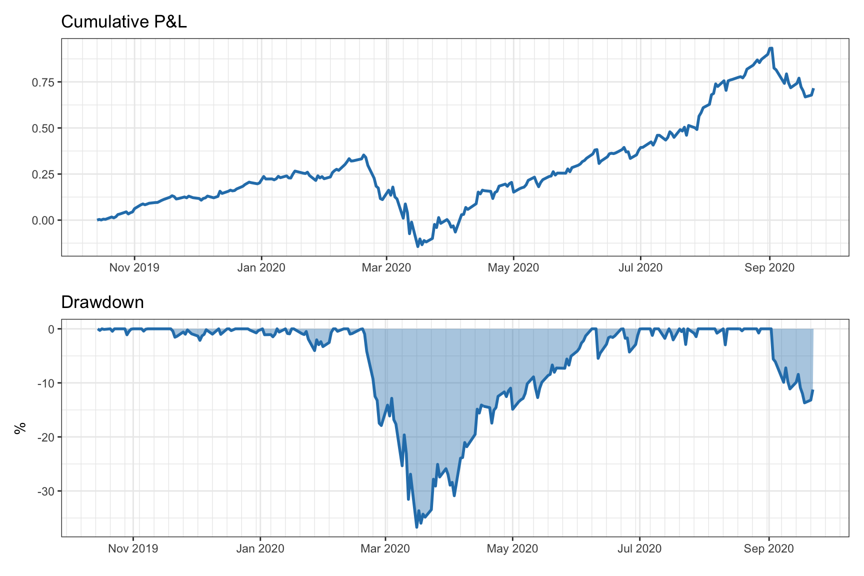
Figure 6.11: Cumulative P&L and corresponding drawdown of a portfolio.
It is interesting to notice that the drawdown is a path-dependent measure, as opposed to all the previously considered measures of performance. This means that it depends on the temporal order in which the returns \(\bm{r}_t\) happen. This is in sharp contrast to the previously considered measures which are agnostic to the ordering of the returns.
In practice, it is useful to condense the entire drawdown curve for a given period \(t=1,\ldots,T\) into a single numerical value. This can be done in different ways, namely:
- maximum drawdown (Max-DD): \[\textm{Max-DD} = \underset{1\le t\le T}{\textm{max}} \;\bar{D}_t;\]
- average drawdown (Ave-DD): \[\textm{Ave-DD} = \frac{1}{T}\sum_{1\le t\le T} \bar{D}_t;\]
- conditional drawdown at risk (CDaR) (defined similarly to the CVaR): \[\textm{CDaR}_{\alpha} = \E\left[\bar{D}_t \mid \bar{D}_t\geq\textm{VaR}_{\alpha}\right],\] where \(\textm{VaR}_{\alpha}\) is the value at risk of the drawdown \(\bar{D}_t\) with confidence level \(\alpha\).
6.3.12 Calmar Ratio and Sterling Ratio
The Calmar ratio modifies the Sharpe ratio by replacing the variance in the denominator with the maximum drawdown: \[\textm{Calmar ratio} = \frac{\w^\T\bmu - r_\textm{f}}{\textm{Max-DD}}.\]
The Sterling ratio is similar to the Calmar ratio except that it adds an excess risk measure to the maximum drawdown (typically of 10%): \[\textm{Sterling ratio} = \frac{\w^\T\bmu - r_\textm{f}}{\textm{Max-DD} + 0.1}.\]