14.2 Robust Portfolio Optimization
After a brief introduction to robust optimization, we will illustrate its application to portfolio design based on the mean–variance formulation, although the techniques can be applied to other portfolio formulations.
14.2.1 Robust Optimization
Consider a general mathematical optimization problem with optimization variable \(\bm{x}\) making explicit the dependency of the functions on the parameter \(\bm{\theta}\): \[ \begin{array}{ll} \underset{\bm{x}}{\textm{minimize}} & \begin{array}[t]{l} f_{0}(\bm{x}; \bm{\theta}) \end{array}\\ \textm{subject to} & \begin{array}[t]{l} f_{i}(\bm{x}; \bm{\theta})\leq0,\\ h_{i}(\bm{x}; \bm{\theta})=0, \end{array} \quad \begin{array}[t]{l} i=1,\ldots,m,\\ i=1,\ldots,p, \end{array} \end{array} \]
where \(f_{0}\) is the objective function, \(f_{i},\; i=1,\ldots,m,\) are the inequality constraint functions, and \(h_{i},\; i=1,\ldots,p,\) are the equality constraint functions. The parameter \(\bm{\theta}\) is something given externally and not to be optimized. For example, in the case of the mean–variance portfolio, we have \(\bm{\theta}=(\bmu, \bSigma)\). We denote a solution to this problem by \(\bm{x}^\star(\bm{\theta})\), where the dependency on \(\bm{\theta}\) is again made explicit.
In practice, however, \(\bm{\theta}\) is unknown and has to be estimated as \(\hat{\bm{\theta}}\). The problem, of course, is that the solution obtained by solving the optimization problem using the estimated \(\hat{\bm{\theta}}\), denoted by \(\bm{x}^\star(\hat{\bm{\theta}})\), differs from the desired one: \(\bm{x}^\star(\hat{\bm{\theta}}) \neq \bm{x}^\star(\bm{\theta})\). The question is whether it is still approximately equal, \(\bm{x}^\star(\hat{\bm{\theta}}) \approx \bm{x}^\star(\bm{\theta})\), or totally different. The answer depends on each particular problem formulation; for the mean–variance portfolio formulation it turns out to be quite different (as illustrated in Figure 14.1).
There are several ways to make the problem robust to parameter errors:
Stochastic optimization relies on a probabilistic modeling of the parameter (Birge and Louveaux, 2011; Prekopa, 1995; Ruszczynski and Shapiro, 2003) and may include:
- expectations: average behavior;
- chance constraints: probabilistic constraints.
Worst-case robust optimization relies on the definition of an uncertainty set for the parameter (Ben-Tal et al., 2009; Ben-Tal and Nemirovski, 2008; Bertsimas et al., 2011; Lobo, 2000).
Stochastic Optimization
In stochastic robust optimization, the estimated parameter \(\hat{\bm{\theta}}\) is modeled as a random variable that fluctuates around its true value \(\bm{\theta}\). For convenience, the true value is modeled as a random variable around the estimated value (with an additive noise) as \[ \bm{\theta} = \hat{\bm{\theta}} + \bm{\delta}, \] where \(\bm{\delta}\) is the estimation error modeled as a zero-mean random variable with some distribution such as Gaussian. In practice, it is critical to choose the covariance matrix (or shape) of the error term properly.
Then, rather than using a naive and wrong constraint of the form \[ f\big(\bm{x}; \hat{\bm{\theta}}\big) \le \alpha, \] we can use the “average constraint” \[ \E_{\bm{\theta}}\left[f(\bm{x}; \bm{\theta})\right] \le \alpha, \] where the expectation is with respect to the random variable \(\bm{\theta}\). The interpretation is that the constraint will be satisfied on average, which is a relaxation of the true constraint.
It is important to point out that this stochastic average constraint preserves convexity. That is, if \(f(\cdot; \bm{\theta})\) is convex for each \(\bm{\theta}\), then its expected value over \(\bm{\theta}\) is also convex (the sum of convex functions preserves convexity, see Appendix A for details).
In practice, the expected value can be implemented in different ways, for example:
- brute-force sampling: simply sample the random variable \(\bm{\theta}\) \(S\) times and use the constraint \[ \frac{1}{S}\sum_{i=1}^S f(\bm{x}; \bm{\theta}_i) \le \alpha; \]
- adaptive sampling: sample the random variable \(\bm{\theta}\) in a smart and efficient way at each iteration while the problem is being solved;
- closed-form expression: compute the expected value in closed form whenever possible (see Example 14.1);
- stochastic programming: a wide variety of numerical methods have been developed for stochastic optimization under the umbrella of stochastic programming (Birge and Louveaux, 2011; Prekopa, 1995; Ruszczynski and Shapiro, 2003).
Example 14.1 (Stochastic average constraint in closed form) Suppose we have the quadratic constraint \(f(\bm{x}; \bm{\theta}) = (\bm{c}^\T\bm{x})^2\), where the parameter is \(\bm{\theta} = \bm{c}\), modeled as \(\bm{c} = \hat{\bm{c}} + \bm{\delta}\), where \(\bm{\delta}\) is zero-mean with covariance matrix \(\bm{Q}\). Then the expected value is \[ \begin{aligned} \E_{\bm{\theta}}\left[f(\bm{x}; \bm{\theta})\right] &= \E_{\bm{\delta}}\left[\left((\hat{\bm{c}} + \bm{\delta})^\T\bm{x}\right)^2\right]\\ &= \E_{\bm{\delta}}\left[(\hat{\bm{c}}^\T\bm{x})^2 + \bm{x}^\T \bm{\delta} \bm{\delta}^\T \bm{x}\right]\\ &= (\hat{\bm{c}}^\T\bm{x})^2 + \bm{x}^\T \bm{Q} \bm{x}, \end{aligned} \] which, interestingly, has the form of the naive version plus a quadratic regularization term.
The problem with expectations and satisfying constraints on average is that there is no control about any specific realization of the estimation error. This relaxed control may not be acceptable in many applications as the constraint will be violated in many instances. The worst-case approach (considered later) tries to deal with this issue, but it may be too conservative. Chance constraints attempt to achieve a compromise between being too relaxed or overly conservative. They are also based on a statistical modeling of the estimation error, but instead of focusing on the average they focus on satisfying the constraint with some high probability (say, 95% of the cases). In this approach, the naive constraint \(f(\bm{x}; \hat{\bm{\theta}}) \le \alpha\) is replaced with \[ \textm{Pr}\left[ f(\bm{x}; \bm{\theta}) \le \alpha \right] \ge \epsilon, \] where \(\epsilon\) is the confidence level, say, \(\epsilon=0.95\) for 95%. Unfortunately, chance or probabilistic constraints are generally very hard to deal with and one typically has to resort to approximations (Ben-Tal et al., 2009; Ben-Tal and Nemirovski, 2008).
Worst-Case Robust Optimization
In worst-case robust optimization, the parameter \(\bm{\theta}\) is not characterized statistically. Instead, it is assumed to lie within an uncertainty region near the estimated value: \[ \bm{\theta} \in \mathcal{U}_{\bm{\theta}}, \] where \(\mathcal{U}_{\bm{\theta}}\) is the uncertainty set centered at \(\hat{\bm{\theta}}\).
In practice, it is critical to choose the shape and size of the uncertainty set properly. Typical choices for the shape for a size of \(\epsilon\) are:
- spherical set: \(\quad \mathcal{U}_{\bm{\theta}} = \left\{\bm{\theta} \mid \|\bm{\theta} - \hat{\bm{\theta}}\|_2 \le \epsilon\right\};\)
- box set: \(\quad \mathcal{U}_{\bm{\theta}} = \left\{\bm{\theta} \mid \|\bm{\theta} - \hat{\bm{\theta}}\|_\infty \le \epsilon\right\};\)
- ellipsoidal set: \(\quad \mathcal{U}_{\bm{\theta}} = \left\{\bm{\theta} \mid \big(\bm{\theta} - \hat{\bm{\theta}}\big)^\T\bm{S}^{-1}\big(\bm{\theta} - \hat{\bm{\theta}}\big) \le \epsilon^2\right\},\) where \(\bm{S}\succ\bm{0}\) defines the shape of the ellipsoid.
Then, rather than using a naive and wrong constraint of the form \[ f\big(\bm{x}; \hat{\bm{\theta}}\big) \le \alpha, \] we can use the worst-case constraint \[ \underset{\bm{\theta} \in \mathcal{U}_{\hat{\bm{\theta}}}}{\textm{sup}} \; f(\bm{x}; \bm{\theta}) \le \alpha. \] The interpretation is that the constraint will be satisfied for any point inside the uncertainty set, which is a conservative approach.
It is important to point out that this worst-case constraint preserves convexity. That is, if \(f(\cdot; \bm{\theta})\) is convex for each \(\bm{\theta}\), then its worst case over \(\bm{\theta}\) is also convex (the pointwise maximum of convex functions preserves convexity, see Appendix A for details).
In practice, the expected value can be implemented in different ways, for example:
- brute-force sampling: simply sample the uncertainty set \(\mathcal{U}_{\bm{\theta}}\) \(S\) times and use the constraint \[ \underset{i=1,\dots,S}{\textm{max}} \; f(\bm{x}; \bm{\theta}_i) \le \alpha \] or, equivalently, include \(S\) constraints \[ f(\bm{x}; \bm{\theta}_i) \le \alpha, \qquad i=1,\dots,S; \]
- adaptive sampling algorithms: sample the uncertainty set \(\mathcal{U}_{\hat{\bm{\theta}}}\) in a smart and efficient way at each iteration while the problem is being solved;
- closed-form expression: compute the supremum in closed form whenever possible (see Example 14.2);
- via Lagrange duality: in some cases, it is possible to rewrite the worst-case supremum as an infimum that can later be combined with the outer portfolio optimization layer;
- saddle-point optimization: as a last resort, since the worst-case design is expressed in the form of a min–max (minimax) formulation, numerical methods specifically designed for minimax problems or related saddle-point problems can be used (Bertsekas, 1999; Tütüncü and Koenig, 2004).
Example 14.2 (Worst-case constraint in closed form) Suppose we have the quadratic constraint \(f(\bm{x}; \bm{\theta}) = (\bm{c}^\T\bm{x})^2\), where the parameter is \(\bm{\theta} = \bm{c}\) and belongs to a spherical uncertainty set \[\mathcal{U} = \left\{\bm{c} \mid \|\bm{c} - \hat{\bm{c}}\|_2 \le \epsilon\right\}.\] Then, the worst-case value is \[ \begin{aligned} \underset{\bm{c} \in \mathcal{U}}{\textm{sup}} \; |\bm{c}^\T\bm{x}| &= \underset{\|\bm{\delta}\| \le \epsilon}{\textm{sup}} \; |(\hat{\bm{c}} + \bm{\delta})^\T\bm{x}| \\ &= |\hat{\bm{c}}^\T\bm{x}| + \underset{\|\bm{\delta}\| \le \epsilon}{\textm{sup}} \; |\bm{\delta}^\T\bm{x}| \\ &= |\hat{\bm{c}}^\T\bm{x}| + \epsilon \|\bm{x}\|_2, \end{aligned} \] where we have used the triangle inequality and the Cauchy–Schwarz inequality (with upper bound achieved by \(\bm{\delta} = \epsilon \, \bm{x}/\|\bm{x}\|_2\)). Again, this expression has the form of the naive version plus a regularization term.
As a final note, it is worth mentioning that worst-case uncertainty philosophy can be applied to probability distributions, referred to as distributional uncertainty models or distributionally robust optimization (Bertsimas et al., 2011).
14.2.2 Robust Worst-Case Portfolios
For portfolio design, we will focus on the worst-case robust optimization philosophy, due to its simplicity and convenience (Goldfarb and Iyengar, 2003; Lobo, 2000; Tütüncü and Koenig, 2004); see also textbooks such as Cornuejols and Tütüncü (2006) and Fabozzi et al. (2007).
Worst-Case Mean Vector \(\bmu\)
To study the uncertainty in \(\bmu\), we consider the global maximum return portfolio (GMRP) for an estimated mean vector \(\hat{\bmu}\) (see Chapter 6 for details): \[ \begin{array}{ll} \underset{\w}{\textm{maximize}} & \w^\T\hat{\bmu}\\ \textm{subject to} & \bm{1}^\T\w=1, \quad \w\ge\bm{0}, \end{array} \] which is is known to be terribly sensitive to estimation errors.
We will instead use the worst-case formulation: \[ \begin{array}{ll} \underset{\w}{\textm{maximize}} & \textm{inf}_{\bmu \in \mathcal{U}_{\bmu}} \; \w^\T\bmu\\ \textm{subject to} & \bm{1}^\T\w=1, \quad \w\ge\bm{0}, \end{array} \] where typical choices for the uncertainty region \(\mathcal{U}_{\bmu}\) are the ellipsoidal and box sets considered next.
Lemma 14.1 (Worst-case mean vector under ellipsoidal uncertainty set) Consider the ellipsoidal uncertainty set for \(\bmu\) \[ \mathcal{U}_{\bmu} = \left\{\bmu = \hat{\bmu} + \kappa \bm{S}^{1/2}\bm{u} \mid \|\bm{u}\|_2 \le 1\right\}, \] where \(\bm{S}^{1/2}\) is the symmetric square-root matrix of the shape \(\bm{S}\) (a typical choice is the covariance matrix scaled with the number of observations, \(\bm{S}=(1/T)\bSigma\)) and \(\kappa\) determines the size of the ellipsoid. Then, the worst-case value of \(\w^\T\bmu\) is \[ \begin{aligned} \underset{\bmu \in \mathcal{U}_{\bmu}}{\textnormal{inf}} \; \w^\T\bmu &= \underset{\|\bm{u}\| \le 1}{\textnormal{inf}} \; \w^\T( \hat{\bmu} + \kappa \bm{S}^{1/2}\bm{u}) \\ &= \w^\T\hat{\bmu} + \kappa\; \underset{\|\bm{u}\| \le 1}{\textnormal{inf}} \; \w^\T\bm{S}^{1/2}\bm{u} \\ &= \w^\T\hat{\bmu} - \kappa\; \|\bm{S}^{1/2}\w\|_2, \end{aligned} \] which follows from the Cauchy–Schwarz inequality with \(\bm{u} = -\bm{S}^{1/2}\w/\|\bm{S}^{1/2}\w\|_2\).
Lemma 14.2 (Worst-case mean vector under box uncertainty set) Consider the box uncertainty set for \(\bmu\) \[ \mathcal{U}_{\bmu} = \left\{\bmu \mid -\bm{\delta} \le \bmu - \hat{\bmu} \le \bm{\delta}\right\}, \] where \(\bm{\delta}\) is the half-width of the box in all dimensions. Then, the worst-case value of \(\w^\T\bmu\) is \[ \begin{aligned} \underset{\bmu \in \mathcal{U}_{\bmu}}{\textnormal{inf}} \; \w^\T\bmu &= \w^\T\hat{\bmu} - |\w|^\T\bm{\delta}, \end{aligned} \] where \(|\w|\) denotes the elementwise absolute value of \(\w\).
Thus, under an ellipsoidal uncertainty set as in Lemma 14.1, the robust version of the GMRP is \[ \begin{array}{ll} \underset{\w}{\textm{maximize}} & \w^\T\hat{\bmu} - \kappa\; \|\bm{S}^{1/2}\w\|_2\\ \textm{subject to} & \bm{1}^\T\w=1, \quad \w\ge\bm{0}, \end{array} \] which is still a convex problem but now the problem complexity has increased to that of a second-order cone program (from a simple linear program in the naive formulation).
Similarly, under a box uncertainty set as in Lemma 14.2, the robust version of the GMRP is \[ \begin{array}{ll} \underset{\w}{\textm{maximize}} & \w^\T\hat{\bmu} - |\w|^\T\bm{\delta}\\ \textm{subject to} & \bm{1}^\T\w=1, \quad \w\ge\bm{0}, \end{array} \] which is still a convex problem and can be rewritten as a linear program after getting rid of the absolute value (see Appendix A for details). In fact, under the constraints \(\bm{1}^\T\w=1\) and \(\w\ge\bm{0}\), the problem can be reduced to a naive GMRP where \(\hat{\bmu}\) is replaced by \(\hat{\bmu} - \bm{\delta}\).
There are other uncertainty sets that can also be considered, such as the \(\ell_1\)-norm ball. The following example illustrates a rather interesting case of how the otherwise heuristic quintile portfolio (see Section 6.4.4 in Chapter 6 for details) can be formally derived as a robust portfolio.
Example 14.3 (Quintile portfolio as a robust portfolio) The quintile portfolio is a heuristic portfolio widely used by practitioners (see Section 6.4.4 in Chapter 6 for details). It selects the top fifth of the assets (one could also select a different fraction of the assets) over which the capital is equally allocated. This is a common-sense heuristic portfolio widely used in practice. Interestingly, it can be shown to be the optimal solution to the worst-case GMRP with an \(\ell_1\)-norm ball uncertainty set around the estimated mean vector (Zhou and Palomar, 2020): \[ \mathcal{U}_{\bmu} = \left\{\hat{\bmu} + \bm{e} \mid \|\bm{e}\|_1 \leq \epsilon\right\}. \]
Worst-Case Covariance Matrix \(\bSigma\)
To study the uncertainty in \(\bSigma\), we consider the global minimum variance portfolio (GMVP) for an estimated mean vector \(\hat{\bSigma}\) (see Chapter 6 for details): \[ \begin{array}{ll} \underset{\w}{\textm{minimize}} & \w^\T\hat{\bSigma}\w\\ \textm{subject to} & \bm{1}^\T\w=1, \quad \w\ge\bm{0}, \end{array} \] which is sensitive to estimation errors (albeit not as much as the previous sensitivity to errors in \(\bmu\)).
We will instead use the worst-case formulation: \[ \begin{array}{ll} \underset{\w}{\textm{minimize}} & \textm{sup}_{\bSigma \in \mathcal{U}_{\bSigma}} \; \w^\T\bSigma\w\\ \textm{subject to} & \bm{1}^\T\w=1, \quad \w\ge\bm{0}, \end{array} \] where typical choices for the uncertainty region \(\mathcal{U}_{\bSigma}\) are the spherical, ellipsoidal, and box sets considered next.
Lemma 14.3 (Worst-case covariance matrix under a data spherical uncertainty set) Consider the spherical uncertainty set for the data matrix \(\bm{X}\in\R^{T\times N}\) containing \(T\) observations of the \(N\) assets, \[ \mathcal{U}_{\bm{X}} = \left\{\bm{X} \mid \|\bm{X} -\hat{\bm{X}}\|_\textnormal{F} \le \epsilon\right\}, \] where \(\epsilon\) determines the size of the sphere. Then, the worst-case value of \(\sqrt{\w^\T\bSigma\w}\) under a sample covariance matrix estimation \(\hat{\bSigma} = \frac{1}{T}\hat{\bm{X}}^\T\hat{\bm{X}}\) is \[ \begin{aligned} \underset{\bm{X} \in \mathcal{U}_{\bm{X}}}{\textnormal{sup}} \; \sqrt{\w^\T\left(\frac{1}{T}\bm{X}^\T\bm{X}\right)\w} &= \underset{\bm{X} \in \mathcal{U}_{\bm{X}}}{\textnormal{sup}} \; \frac{1}{\sqrt{T}} \|\bm{X}\w\|_2\\ &= \underset{\|\bm{\Delta}\|_\textnormal{F} \le \epsilon}{\textnormal{sup}} \; \frac{1}{\sqrt{T}} \left\|(\hat{\bm{X}} + \bm{\Delta})\w\right\|_2\\ &= \frac{1}{\sqrt{T}} \left\|\hat{\bm{X}}\w\right\|_2 + \underset{\|\bm{\Delta}\|_\textnormal{F} \le \epsilon}{\textnormal{sup}} \; \frac{1}{\sqrt{T}} \left\|\bm{\Delta}\w\right\|_2\\ &= \frac{1}{\sqrt{T}} \left\|\hat{\bm{X}}\w\right\|_2 + \frac{1}{\sqrt{T}} \epsilon \|\w\|_2, \end{aligned} \] where the third equality follows from the triangle inequality and is achieved when \(\hat{\bm{X}}\w\) and \(\bm{\Delta}\w\) are aligned.
Lemma 14.4 (Worst-case covariance matrix under an ellipsoidal uncertainty set) Consider the ellipsoidal uncertainty set for \(\bSigma\) \[ \mathcal{U}_{\bSigma} = \left\{\bSigma \succeq \bm{0} \mid \big(\textnormal{vec}(\bSigma) - \textnormal{vec}(\hat{\bSigma})\big)^\T \bm{S}^{-1} \big(\textnormal{vec}(\bSigma) - \textnormal{vec}(\hat{\bSigma})\big) \le \epsilon^2\right\}, \] where \(\textnormal{vec}(\cdot)\) denotes the operator that stacks the matrix argument into a vector, matrix \(\bm{S}\) gives the shape of the ellipsoid, and \(\epsilon\) determines the size. Then, the worst-case value of \(\w^\T\bSigma\w\) given by the convex semidefinite problem \[ \begin{array}{ll} \underset{\bSigma}{\textm{maximize}} & \w^\T\bSigma\w\\ \textm{subject to} & \big(\textnormal{vec}(\bSigma) - \textnormal{vec}(\hat{\bSigma})\big)^\T \bm{S}^{-1} \big(\textnormal{vec}(\bSigma) - \textnormal{vec}(\hat{\bSigma})\big) \le \epsilon^2\\ & \bSigma \succeq \bm{0}, \end{array} \] can be rewritten as the Lagrange dual problem: \[ \begin{array}{ll} \underset{\bm{Z}}{\textm{minimize}} & \textnormal{Tr}\left(\hat{\bSigma}\left(\w\w^\T+\bm{Z}\right)\right) + \epsilon\left\| \bm{S}^{1/2}\left(\textnormal{vec}(\w\w^\T)+\textnormal{vec}(\bm{Z})\right)\right\|_{2}\\ \textm{subject to} & \bm{Z} \succeq \bm{0}, \end{array} \] which is a convex semidefinite problem.
Lemma 14.5 (Worst-case covariance matrix under a box uncertainty set) Consider the box uncertainty set for \(\bSigma\) \[ \mathcal{U}_{\bSigma} = \left\{\bSigma \succeq \bm{0} \mid \underline{\bSigma} \le \bSigma \le \overline{\bSigma}\right\}, \] where \(\underline{\bSigma}\) and \(\overline{\bSigma}\) denote the elementwise lower and upper bounds, respectively. Then, the worst-case value of \(\w^\T\bSigma\w\), given by the convex semidefinite problem \[ \begin{array}{ll} \underset{\bSigma}{\textm{maximize}} & \w^\T\bSigma\w\\ \textm{subject to} & \underline{\bSigma} \le \bSigma \le \overline{\bSigma},\\ & \bSigma \succeq \bm{0}, \end{array} \] can be rewritten as the Lagrange dual problem (Lobo, 2000) \[ \begin{array}{ll} \underset{\overline{\bm{\Lambda}},\,\underline{\bm{\Lambda}}}{\textm{minimize}} & \textnormal{Tr}\big(\overline{\bm{\Lambda}}\,\overline{\bSigma}\big) - \textnormal{Tr}\big(\underline{\bm{\Lambda}}\,\underline{\bSigma}\big)\\ \textm{subject to} & \begin{bmatrix} \overline{\bm{\Lambda}} - \underline{\bm{\Lambda}} & \w\\ \w^\T & 1 \end{bmatrix} \succeq \bm{0}\\ & \overline{\bm{\Lambda}}\geq\bm{0},\quad\underline{\bm{\Lambda}}\geq\bm{0}, \end{array} \] which is a convex semidefinite problem.
Thus, under a spherical uncertainty set for the data matrix as in Lemma 14.3, the robust version of the GMVP is \[ \begin{array}{ll} \underset{\w}{\textm{minimize}} & \left(\left\|\hat{\bm{X}}\w\right\|_2 + \epsilon \|\w\|_2\right)^2\\ \textm{subject to} & \bm{1}^\T\w=1, \quad \w\ge\bm{0}, \end{array} \] which is still a convex problem but now the problem complexity has increased to that of a second-order cone program (from a simple quadratic program in the naive formulation).
Interestingly, this problem bears a striking resemblance to a common heuristic called Tikhonov regularization: \[ \begin{array}{ll} \underset{\w}{\textm{minimize}} & \left\|\hat{\bm{X}}\w\right\|_2^2 + \epsilon \|\w\|_2^2\\ \textm{subject to} & \bm{1}^\T\w=1, \quad \w\ge\bm{0}, \end{array} \] where the objective function can be rewritten as \(\w^\T\frac{1}{T}\big(\hat{\bm{X}}^\T\hat{\bm{X}} + \epsilon \bm{I}\big)\w\), which leads to a regularized sample covariance matrix (see Section 3.6.1 in Chapter 3 for details on shrinkage).
Regarding the worst-case formulations that involve the Lagrange dual problem, the outer and inner minimizations can be simply written as a joint minimization. For example, under an ellipsoidal uncertainty set for the covariance matrix as in Lemma 14.4, the robust version of the GMVP is (Feng and Palomar, 2016) \[ \begin{array}{ll} \underset{\w,\bm{W},\bm{Z}}{\textm{minimize}} & \textm{Tr}\left(\hat{\bSigma}\left(\bm{W}+\bm{Z}\right)\right) + \epsilon\left\| \bm{S}^{1/2}\left(\textm{vec}(\bm{W})+\textm{vec}(\bm{Z})\right)\right\|_{2}\\ \textm{subject to} & \begin{bmatrix} \bm{W} & \w\\ \w^\T & 1 \end{bmatrix} \succeq \bm{0}\\ & \bm{1}^\T\w=1, \quad \w\ge\bm{0},\\ & \bm{Z} \succeq \bm{0}, \end{array} \] which is still a convex problem but now the problem complexity has increased to that of a semidefinite program (from a simple quadratic program in the naive formulation). Note that the first matrix inequality is equivalent to \(\bm{W}\succeq\w\w^\T\) and, at an optimal point, it can be shown to be satisfied with equality \(\bm{W}=\w\w^\T\).
Worst-Case Mean Vector \(\bmu\) and Covariance Matrix \(\bSigma\)
The previous worst-case formulations against uncertainty in the mean vector \(\bmu\) and the covariance matrix \(\bSigma\) can be trivially combined under the mean–variance portfolio formulation.
For illustrative purposes, we consider the the mean–variance worst-case portfolio formulation under box uncertainty sets for \(\bmu\) and \(\bSigma\), as in Lemmas 14.2 and 14.5, given by \[ \begin{array}{ll} \underset{\w,\,\overline{\bm{\Lambda}},\,\underline{\bm{\Lambda}}}{\textm{maximize}} & \w^\T\hat{\bmu} - |\w|^\T\bm{\delta} - \frac{\lambda}{2} \left( \textm{Tr}\big(\overline{\bm{\Lambda}}\,\overline{\bSigma}\big) - \textm{Tr}\big(\underline{\bm{\Lambda}}\,\underline{\bSigma}\big) \right)\\ \textm{subject to} & \bm{1}^\T\w=1, \quad \w\ge\bm{0},\\ & \begin{bmatrix} \overline{\bm{\Lambda}} - \underline{\bm{\Lambda}} & \w\\ \w^\T & 1 \end{bmatrix} \succeq \bm{0},\\ & \overline{\bm{\Lambda}}\geq\bm{0},\quad\underline{\bm{\Lambda}}\geq\bm{0}, \end{array} \] which is a convex semidefinite problem.
Other more sophisticated uncertainty sets can be considered for the mean vector and the covariance matrix, such as based on factor modeling (Goldfarb and Iyengar, 2003).
Other Worst-Case Performance Measures
Apart from the mean–variance framework for portfolio optimization, many other portfolio designs can be formulated based on other objective functions or performance measures (see Chapter 10 for details), as well as higher-order moments (see Chapter 9) or risk-parity portfolios (see Chapter 11). Each such formulation can be robustified so that the solution becomes more stable and robust against estimation errors in the parameters. For example, the worst-case Sharpe ratio can be easily managed, as well as the the worst-case value-at-risk (VaR) (El Ghaoui et al., 2003).
14.2.3 Numerical Experiments
The effectiveness of the different robust portfolio formulations depends on the shape as well as the size of the uncertainty region. These are parameters that have to be properly chosen and tuned to the type of data and nature of the financial market. Therefore, it is easy to overfit the model to the training data and extra care has to be taken.
The goal of a robust design should be in making the solution more stable and less sensitive to the error realization, but not necessarily improving the performance. In other words, one should aim at gaining robustness but not the best performance for a given backtest compared to a naive design.
We now evaluate robust portfolios under errors in the mean vector \(\bmu\). Recall that robustness for the covariance matrix \(\bSigma\) is not as critical, because the bottleneck in the estimation part is on the mean vector (see Chapter 3 for details).
Sensitivity of Robust Portfolios
The extreme sensitivity of a naive mean–variance portfolio was shown in Figure 14.1. We now repeat the same numerical experiment with a robust formulation (still with \(\lambda=1\)).
Figure 14.2 shows the sensitivity of a robust portfolio under an ellipsoidal uncertainty set for the mean vector \(\bmu\) over six different realizations of the estimation error. Compared to Figure 14.1, it is clearly more stable and less sensitive. Many other variations in the robust formulation can be similarly considered with similar results.
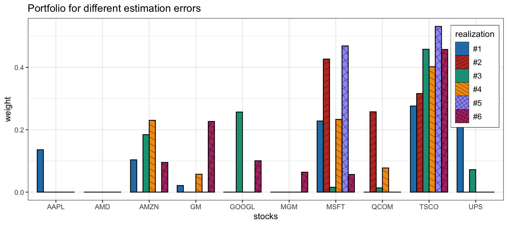
Figure 14.2: Sensitivity of the robust mean–variance portfolio under an ellipsoidal uncertainty set for \(\bm{\mu}\).
Comparison of Naive vs. Robust Portfolios
Now that we have empirically observed the improved stability of mean–variance robust designs, we can assess their performance (with box and ellipsoidal uncertainty sets for the mean vector \(\bmu\)) in comparison with the naive design. Backtests are conducted for 50 randomly chosen stocks from the S&P 500 during 2017–2020.
Figure 14.3 shows the empirical distribution of the achieved mean–variance objective, as well as the Sharpe ratio, calculated over 1,000 Monte Carlo noisy observations. We can see that the robust designs avoid the worst-case realizations (the left tail in the distributions) at the expense of not achieving the best-case realizations (the right tail); thus, they are more stable and robust as expected.
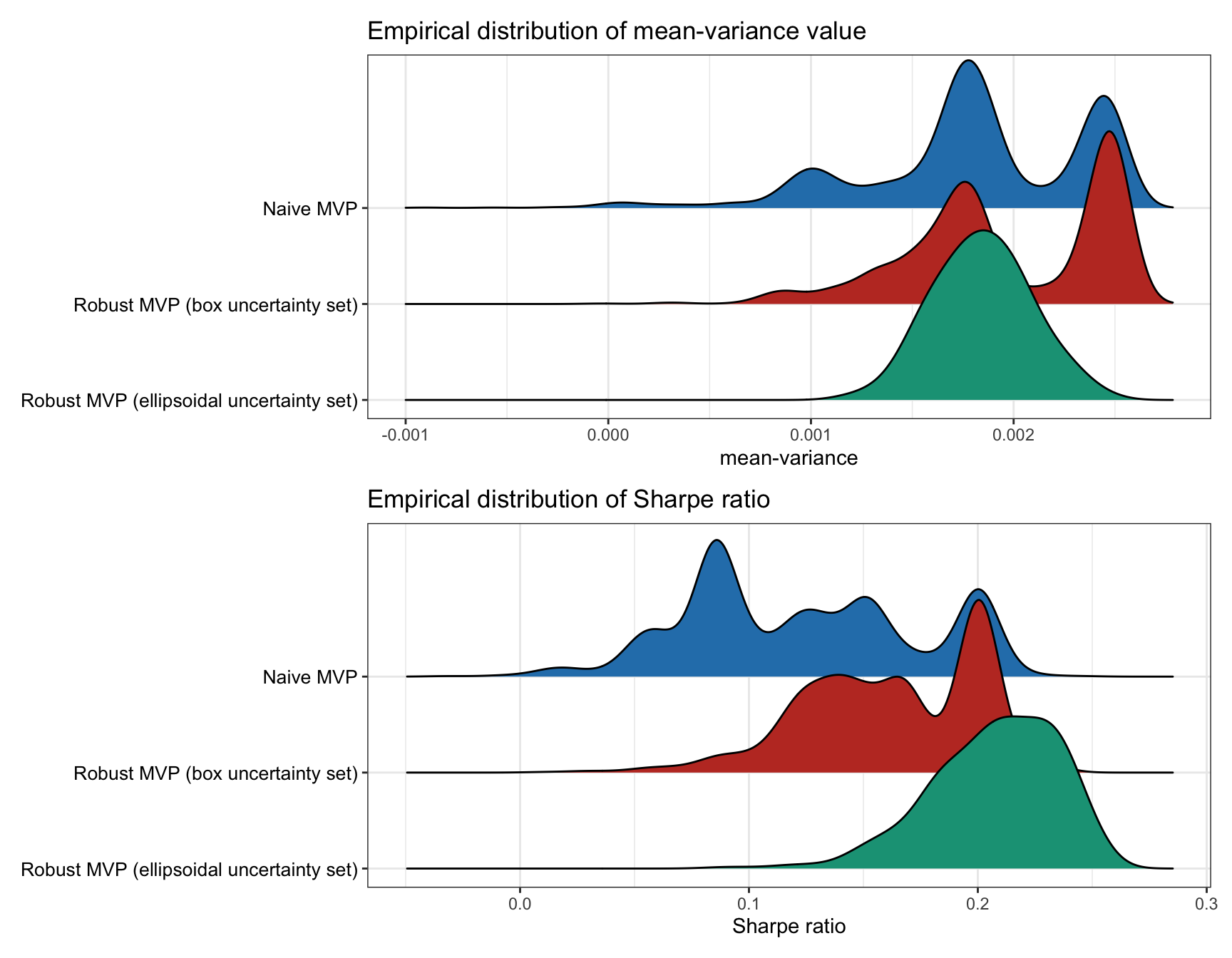
Figure 14.3: Empirical performance distribution of naive vs. robust mean–variance portfolios.
Figure 14.4 shows the cumulative return and drawdown of the naive and robust mean–variance portfolios for an illustrative backtest. We can observe how the robust portfolios do indeed seem to be more robust. However, this is just a single backtest and more exhaustive multiple backtest are necessary.
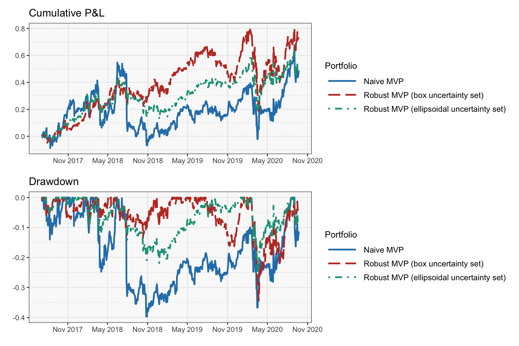
Figure 14.4: Backtest of naive vs. robust mean–variance portfolios.
Finally, multiple backtests are conducted for 200 realizations of 50 randomly chosen stocks from the S&P 500 from random periods during 2015–2020. Figure 14.5 shows the results in terms of the Sharpe ratio and drawdown, confirming that the robust portfolios are superior to the naive portfolio.
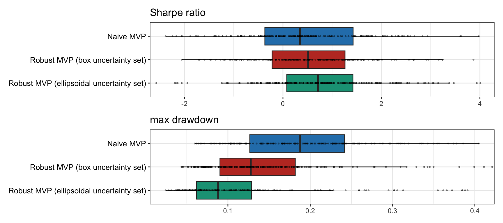
Figure 14.5: Multiple backtests of naive vs. resampled mean–variance portfolios.