B.8 Successive Convex Approximation (SCA)
The successive convex approximation (SCA) method (or framework) approximates a difficult optimization problem by a sequence of simpler convex problems. We now give a brief description. For details, the reader is referred to the original paper, Scutari et al. (2014), and the comprehensive book chapter, Scutari and Sun (2018).
Suppose the following (difficult) problem is to be solved: \[\begin{equation} \begin{array}{ll} \underset{\bm{x}}{\textm{minimize}} & f(\bm{x})\\ \textm{subject to} & \bm{x} \in \mathcal{X}, \end{array} \tag{B.13} \end{equation}\] where \(f\) is the (possibly nonconvex) objective function and \(\mathcal{X}\) is a convex set. Nonconvex sets can also be accommodated at the expense of significantly complicating the method (Scutari and Sun, 2018). Instead of attempting to directly obtain a solution \(\bm{x}^\star\) (either a local or a global solution), the SCA method will produce a sequence of iterates \(\bm{x}^0, \bm{x}^1, \bm{x}^2,\dots\) that will converge to \(\bm{x}^\star\).
More specifically, at iteration \(k\), the SCA approximates the objective function \(f(\bm{x})\) by a surrogate function around the current point \(\bm{x}^k\), denoted by \(\tilde{f}\left(\bm{x};\bm{x}^k\right)\). This surrogate function need not be an upper bound like in MM; in this sense, it is more relaxed. At this point, one may be tempted to solve the sequence of (simpler) problems: \[ \bm{x}^{k+1}=\underset{\bm{x}\in\mathcal{X}}{\textm{arg min}}\;\tilde{f}\left(\bm{x};\bm{x}^k\right), \qquad k=0,1,2,\dots \]
Unfortunately, the previous sequence of updates may not converge and a smoothing step is necessary to introduce some memory in the process, which will avoid undesired oscillations. Thus, the correct sequence of problems for the SCA method is \[ \begin{array}{ll} \left. \begin{aligned} \hat{\bm{x}}^{k+1} &= \underset{\bm{x}\in\mathcal{X}}{\textm{arg min}}\;\tilde{f}\left(\bm{x};\bm{x}^k\right)\\ \bm{x}^{k+1} &= \bm{x}^{k} + \gamma^k \left(\hat{\bm{x}}^{k+1} - \bm{x}^{k}\right) \end{aligned} \quad \right\} \qquad k=0,1,2,\dots, \end{array} \] where \(\{\gamma^k\}\) is a properly designed sequence with \(\gamma^k \in (0,1]\) (Scutari et al., 2014). This iterative process is illustrated in Figure B.10; observe that the surrogate function is not an upper bound on the original function.

Figure B.10: Illustration of sequence of surrogate problems in SCA.
In order to guarantee convergence of the iterates, the surrogate function \(\tilde{f}\left(\bm{x};\bm{x}^k\right)\) has to satisfy the following technical conditions (Scutari et al., 2014):
- \(\tilde{f}\left(\bm{x};\bm{x}^k\right)\) must be strongly convex on the feasible set \(\mathcal{X}\); and
- \(\tilde{f}\left(\bm{x};\bm{x}^k\right)\) must be differentiable with \(\nabla\tilde{f}\left(\bm{x};\bm{x}^k\right) = \nabla f\left(\bm{x}\right)\).
The sequence \(\{\gamma^k\}\) can be chosen according to different stepsize rules (Scutari et al., 2014; Scutari and Sun, 2018):
- Bounded stepsize: The values \(\gamma^k\) are sufficiently small (difficult to use in practice since the values have to be smaller than some bound which is generally unknown or difficult to compute).
- Backtracking line search: This is effective in terms of iterations, but performing the line search requires evaluating the objective function multiple times per iteration, resulting in more costly iterations.
- Diminishing stepsize: A good practical choice is a sequence satisfying \(\sum_{k=1}^\infty \gamma^k=+\infty\) and \(\sum_{k=1}^\infty (\gamma^k)^2<+\infty\). Two very effective examples of diminishing stepsize rules are: \[ \gamma^{k+1} = \gamma^k\left(1-\epsilon\gamma^k\right),\quad k=0,1,\dots,\quad\gamma^0<1/\epsilon, \] where \(\epsilon\in(0,1)\), and \[ \gamma^{k+1} = \frac{\gamma^k+\alpha^k}{1+\beta^k},\quad k=0,1,\dots,\quad\gamma^0=1, \] where \(\alpha^k\) and \(\beta^k\) satisfy \(0\le\alpha^k\le\beta^k\) and \(\alpha^k/\beta^k\to0\) as \(k\to\infty\) while \(\sum_k\alpha^k/\beta^k=\infty\). Examples of such \(\alpha^k\) and \(\beta^k\) are: \(\alpha^k=\alpha\) or \(\alpha^k=\textm{log}(k)^\alpha\), and \(\beta^k=\beta k\) or \(\beta^k=\beta \sqrt{k}\), where \(\alpha\) and \(\beta\) are given constants satisfying \(\alpha\in(0,1),\) \(\beta\in(0,1),\) and \(\alpha\le\beta\).
SCA takes its name from the fact that the surrogate function is convex by construction. Differently from MM, constructing a convex surrogate function is not difficult. This facilitates the use of SCA in many applications. SCA can be described very simply, as summarized in Algorithm B.8.
Algorithm B.8: SCA to solve the general problem in (B.13).
Choose initial point \(\bm{x}^0\in\mathcal{X}\) and sequence \(\{\gamma^k\}\);
Set \(k \gets 0\);
repeat
- Construct surrogate of \(f(\bm{x})\) around current point \(\bm{x}^k\) as \(\tilde{f}\left(\bm{x};\bm{x}^k\right)\);
- Obtain intermediate point by solving the surrogate convex problem: \[\hat{\bm{x}}^{k+1} = \underset{\bm{x}\in\mathcal{X}}{\textm{arg min}}\;\tilde{f}\left(\bm{x};\bm{x}^k\right);\]
- Obtain next iterate by averaging the intermediate point with the previous one: \[\bm{x}^{k+1} = \bm{x}^{k} + \gamma^k \left(\hat{\bm{x}}^{k+1} - \bm{x}^{k}\right);\]
- \(k \gets k+1\);
until convergence;
B.8.1 Gradient Descent Method as SCA
Consider the unconstrained problem \[ \begin{array}{ll} \underset{\bm{x}}{\textm{minimize}} & f(\bm{x}). \end{array} \] If we now employ SCA with the surrogate function \[ \tilde{f}\left(\bm{x};\bm{x}^k\right) = f\left(\bm{x}^k\right) + \nabla f\left(\bm{x}^k\right)^\T \left(\bm{x} - \bm{x}^k\right) + \frac{1}{2\alpha^k}\|\bm{x} - \bm{x}^k\|^2, \] then to minimize the convex function \(\tilde{f}\left(\bm{x};\bm{x}^k\right)\) we just need to set its gradient to zero, leading to the solution \(\bm{x} = \bm{x}^k - \alpha^k \nabla f\left(\bm{x}^k\right).\) Thus, the iterations are \[ \bm{x}^{k+1} = \bm{x}^k - \alpha^k \nabla f\left(\bm{x}^k\right), \qquad k=0,1,2,\dots, \] which coincides with the gradient descent method.
B.8.2 Newton’s Method as SCA
If we now include the second-order information (i.e., the Hessian of \(f\)) in the surrogate function, \[ \tilde{f}\left(\bm{x};\bm{x}^k\right) = f\left(\bm{x}^k\right) + \nabla f\left(\bm{x}^k\right)^\T \left(\bm{x} - \bm{x}^k\right) + \frac{1}{2\alpha^k}\left(\bm{x} - \bm{x}^k\right)^\T \nabla^2 f\left(\bm{x}^k\right) \left(\bm{x} - \bm{x}^k\right), \] then the resulting iterations are \[ \bm{x}^{k+1} = \bm{x}^k - \alpha^k \nabla^2 f\left(\bm{x}^k\right)^{-1} \nabla f\left(\bm{x}^k\right), \qquad k=0,1,2,\dots, \] which coincides with Newton’s method.
B.8.3 Parallel SCA
While SCA applied to problem (B.13) can be instrumental in devising efficient algorithms, its true potential is realized when the variables can be partitioned into \(n\) blocks \(\bm{x} = (\bm{x}_1,\dots,\bm{x}_n)\) that are separately constrained: \[ \begin{array}{ll} \underset{\bm{x}}{\textm{minimize}} & f(\bm{x}_1,\dots,\bm{x}_n)\\ \textm{subject to} & \bm{x}_i \in \mathcal{X}_i, \qquad i=1,\dots,n. \end{array} \]
In this case, SCA is able to update each of the variables in a parallel fashion (unlike BCD or block MM where the updates are sequential) by using the surrogate functions \(\tilde{f}_i\left(\bm{x}_i;\bm{x}^k\right)\) (Scutari et al., 2014): \[ \begin{array}{ll} \left. \begin{aligned} \hat{\bm{x}}_i^{k+1} &= \underset{\bm{x}_i\in\mathcal{X}_i}{\textm{arg min}}\;\tilde{f}_i\left(\bm{x}_i;\bm{x}^k\right)\\ \bm{x}_i^{k+1} &= \bm{x}_i^{k} + \gamma^k \left(\hat{\bm{x}}_i^{k+1} - \bm{x}_i^{k}\right) \end{aligned} \quad \right\} \qquad i=1,\dots,n, \quad k=0,1,2,\dots \end{array} \]
B.8.4 Convergence
SCA is an extremely versatile framework for deriving practical algorithms. In addition, it enjoys nice theoretical convergence as derived in Scutari et al. (2014) and summarized in Theorem B.5.
Theorem B.5 (Convergence of SCA) Suppose that the surrogate function \(\tilde{f}\left(\bm{x};\bm{x}^k\right)\) (or each \(\tilde{f}_i\left(\bm{x}_i;\bm{x}^k\right)\) in the parallel version) satisfies the previous technical conditions and \(\{\gamma^k\}\) is chosen according to bounded stepsize, diminishing rule, or backtracking line search. Then the sequence \(\{\bm{x}^k\}\) converges to a stationary point of the original problem.
B.8.5 Illustrative Examples
We now describe a few illustrative examples of applications of SCA, along with numerical experiments.
Example B.10 (\(\ell_2\)–\(\ell_1\)-norm minimization via SCA) Consider the \(\ell_2\)–\(\ell_1\)-norm minimization problem \[ \begin{array}{ll} \underset{\bm{x}}{\textm{minimize}} & \frac{1}{2}\|\bm{A}\bm{x} - \bm{b}\|_2^2 + \lambda\|\bm{x}\|_1. \end{array} \]
This problem can be conveniently solved via BCD (see Section B.6), via MM (see Section B.7), or simply by calling a QP solver. We will now develop a simple iterative algorithm based on SCA that leverages the element-by-element closed-form solution.
In this case, we can use parallel SCA by partitioning the variable \(\bm{x}\) into each element \((x_1,\dots,x_n)\) and employing the surrogate functions \[ \tilde{f}\left(\bm{x}_i;\bm{x}^k\right) = \frac{1}{2}\left\|\bm{a}_i x_i - \tilde{\bm{b}}_i^k\right\|_2^2 + \lambda |x_i| + \frac{\tau}{2} \left(x_i - x_i^k\right)^2, \] where \(\tilde{\bm{b}}_i^k = \bm{b} - \sum_{j\neq i}\bm{a}_j x_j^k\).
Therefore, the sequence of surrogate problems to be solved for \(k=0,1,2,\dots\) is \[ \begin{array}{ll} \underset{\bm{x}}{\textm{minimize}} & \frac{1}{2}\left\|\bm{a}_i x_i - \tilde{\bm{b}}_i^k\right\|_2^2 + \lambda |x_i| + \tau \left(x_i - x_i^k\right)^2, \end{array} \qquad i=1,\dots,n, \] with the solution given by the soft-thresholding operator (see Section B.6).
This finally leads to the following SCA iterative algorithm: \[ \begin{array}{ll} \left. \begin{aligned} \hat{x}_i^{k+1} &= \frac{1}{\tau + \|\bm{a}_i\|^2} \mathcal{S}_{\lambda} \left(\bm{a}_i^\T \tilde{\bm{b}}_i^k + \tau x_i^k\right)\\ x_i^{k+1} &= x_i^{k} + \gamma^k \left(\hat{x}_i^{k+1} - x_i^{k}\right) \end{aligned} \quad \right\} \qquad i=1,\dots,n, \quad k=0,1,2,\dots, \end{array} \] where \(\mathcal{S}_{\lambda}(\cdot)\) is the soft-thresholding operator defined in (B.11). Figure B.11 shows the convergence of the SCA iterates.
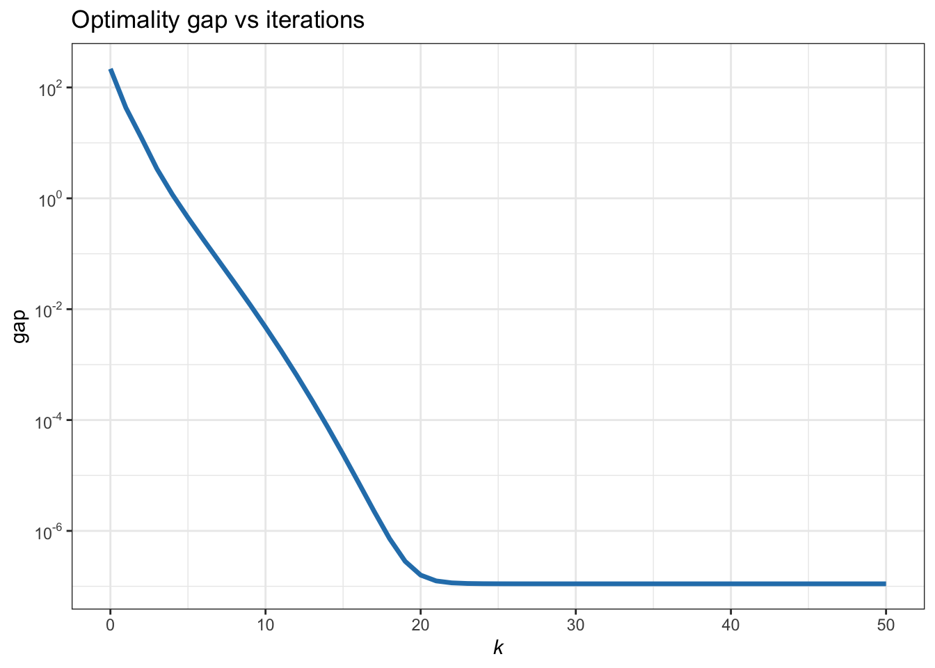
Figure B.11: Convergence of SCA for the \(\ell_2\)–\(\ell_1\)-norm minimization.
Example B.11 (Dictionary learning) Consider the dictionary learning problem: \[ \begin{array}{ll} \underset{\bm{D},\bm{X}}{\textm{minimize}} & \frac{1}{2}\|\bm{Y} - \bm{D}\bm{X}\|_F^2 + \lambda\|\bm{X}\|_1\\ \textm{subject to} & \|[\bm{D}]_{:,i}\| \le 1,\qquad i=1,\dots,m, \end{array} \] where \(\|\bm{D}\|_F\) denotes the matrix Frobenius norm of \(\bm{D}\) (i.e., the \(\ell_2\)-norm of the vectorized form of the matrix or the sum of the squares of all the elements) and \(\|\bm{X}\|_1\) denotes the elementwise \(\ell_1\)-norm of \(\bm{X}\) (i.e., the \(\ell_1\)-norm of the vectorized form of the matrix).
Matrix \(\bm{D}\) is the so-called dictionary and it is a fat matrix that contains a dictionary along the columns that can explain the columns of the data matrix \(\bm{Y}\). Matrix \(\bm{X}\) selects a few columns of the dictionary and, hence, has to be sparse (enforced by the regularizer \(\|\bm{X}\|_1\)).
This problem is not jointly convex in \((\bm{D},\bm{X})\), but it is bi-convex: for a fixed \(\bm{D}\), it is convex in \(\bm{X}\) and, for a fixed \(\bm{X}\), it is convex in \(\bm{D}\). One way to deal with this problem is via BCD (see Section B.6), which would update \(\bm{D}\) and \(\bm{X}\) sequentially. An alternative way is via SCA, which allows a parallel update of \(\bm{D}\) and \(\bm{X}\).
For the SCA approach we can use the following two surrogate functions for \(\bm{D}\) and \(\bm{X}\), respectively: \[ \begin{aligned} \tilde{f}_1\left(\bm{D};\bm{X}^k\right) &= \frac{1}{2}\|\bm{Y} - \bm{D}\bm{X}^k\|_F^2,\\ \tilde{f}_2\left(\bm{X};\bm{D}^k\right) &= \frac{1}{2}\|\bm{Y} - \bm{D}^k\bm{X}\|_F^2. \end{aligned} \] This leads to the following two convex problems:
- A normalized LS problem: \[ \begin{array}{ll} \underset{\bm{D}}{\textm{minimize}} & \frac{1}{2}\|\bm{Y} - \bm{D}\bm{X}^k\|_F^2\\ \textm{subject to} & \|[\bm{D}]_{:,i}\| \le 1,\qquad i=1,\dots,m. \end{array} \]
- A matrix version of the \(\ell_2 - \ell_1\)-norm problem: \[ \begin{array}{ll} \underset{\bm{X}}{\textm{minimize}} & \frac{1}{2}\|\bm{Y} - \bm{D}^k\bm{X}\|_F^2 + \lambda\|\bm{X}\|_1, \end{array} \] which can be further decomposed into a set of vectorized \(\ell_2 - \ell_1\)-norm problems for each column of \(\bm{X}\).
B.8.6 MM vs. SCA
The MM and SCA algorithmic frameworks appear very similar: both are based on solving a sequence of surrogate problems. The difference is in the details, as we compare next.
- Surrogate function: MM requires the surrogate function to be a global upper bound (which can be difficult to derive and too restrictive in some cases), albeit not necessarily convex. On the other hand, SCA relaxes this upper-bound condition in exchange for the requirement of strong convexity. Figure B.12 illustrates the potential benefit of relaxing the upper-bound requirement.

Figure B.12: Illustration of MM vs. SCA: relaxing the upper-bound requirement.
Constraint set: In principle, both SCA and MM require the feasible set \(\mathcal{X}\) to be convex. However, the convergence of MM can be easily extended to nonconvex \(\mathcal{X}\) on a case-by-case basis – refer to the examples in J. Song et al. (2015), Y. Sun et al. (2017), Kumar et al. (2019), and Kumar et al. (2020). SCA cannot deal with a nonconvex \(\mathcal{X}\) directly, although some extensions allow for a successive convexification of \(\mathcal{X}\) at the expense of a much more complex algorithm (Scutari and Sun, 2018).
Schedule of updates: Both MM and SCA can deal with a separable variable \(\bm{x} = (\bm{x}_1,\dots,\bm{x}_n)\). However, block MM requires a sequential update (Razaviyayn et al., 2013; Y. Sun et al., 2017), whereas SCA naturally implements a parallel update, which is more amenable for distributed implementations.