10.2 Alternative Risk Measures
The return obtained by portfolio \(\w\) is \(R = \w^\T\bm{r}\), where \(\bm{r}\) denotes the vector of random returns of the \(N\) assets (see Chapter 6 for details). Since the portfolio return \(R\) is a random variable, a proper full characterization is provided by the probability distribution function (pdf). For simplicity and convenience, the information contained in the pdf is typically condensed into a few key numbers, such as the mean (expected return) and the standard deviation (as a measure of risk). However, determining the appropriate quantity that should be used as a measure of risk has been a subject of scientific investigation since the 1950s (McNeil et al., 2015).
As a consequence, academics and practitioners have explored over decades alternative risk measures that satisfy desirable properties, notably the family of coherent risk measures that satisfy four basic properties: translation invariance, monotonicity, subadditivity, and positive homogeneity (Artzner et al., 1999).
Figure 10.1 illustrates the meaning of the most popular measures of risk in the context of the pdf of the portfolio return, namely, the variance/volatility, the semi-variance/semi-deviation, the VaR, and the CVaR.

Figure 10.1: Illustration of return distribution and measures of risk.
In the following, we describe in detail variations of downside risk, VaR, CVaR, and drawdown. As will be discussed later, drawdown is fundamentally different from all the other measures in that it is not invariant to the order of the returns.
10.2.1 Downside Risk
Economists have long recognized that investors care differently about downside losses vs. upside gains (Roy, 1952). Markowitz himself advocated using the semi-variance as a measure of risk, rather than the variance (Markowitz, 1959).
Downside risk generally refers to risk measures that quantify the losses below a certain threshold. A number of studies indicate that downside risk measures are more meaningful than symmetric measures such as the variance or volatility (Ang et al., 2006; Estrada, 2006). Nevertheless, if the distribution of returns is not sufficiently asymmetric, downside risk measures may not withstand scrutiny in terms of providing an advantage over the variance or volatility (Grootveld and Hallerbach, 1999).
Semi-variance and Semi-deviation
The variance of the return random variable \(R\) is \[ \sigma^2 = \E\left[(R - \mu)^2\right], \] where \(\mu = \E[R]\) is the mean. The semi-variance (SV) is similarly defined but only taking into account when the random variable is below the mean: \[\begin{equation} \textm{SV} = \E\left[\left((\mu - R)^+\right)^2\right], \tag{10.1} \end{equation}\] where the operator \((\cdot)^+ = \textm{max}(0, \cdot)\) only keeps the nonnegative part.
Similarly to the volatility (the square root of the variance), the semi-deviation is defined as the square root of the semi-variance. A related performance measure is the Sortino ratio, defined as the ratio of the expected return to the semi-deviation (similarly to the Sharpe ratio, which uses the volatility instead).
LPM
The lower partial moment (LPM) is a generalization of the semi-variance (Bawa, 1975; Fishburn, 1977): \[\begin{equation} \textm{LPM}_\alpha = \E\left[\left((\tau - R)^+\right)^\alpha\right], \tag{10.2} \end{equation}\] where the parameter \(\tau\) is termed the disaster level (minimum acceptable return) and the parameter \(\alpha\) reflects the investor’s feeling about falling short of \(\tau\), namely, \(\alpha>1\) naturally fits a risk-averse investor, \(\alpha=1\) corresponds to a neutral investor, and \(0<\alpha<1\) is suitable for risk-seeking behavior.
By changing the parameters \(\alpha\) and \(\tau\) in (10.2) most downside measures used in practice can be formed. For instance, setting \(\alpha=2\) and \(\mu = \E[R]\) yields the semi-variance (10.1).
In the same way that in the traditional modern portfolio theory it is common to plot the mean–volatility trade-off achieved by portfolios (see Section 7.1.1 in Chapter 7 for details), we can similarly plot the mean–risk trade-off where the risk is given by \(\textm{LPM}_\alpha^{1/\alpha}\).
10.2.2 Tail Measures: VaR, CVaR, and EVaR
Tail measures, as the name indicates, focus on the tail of the distribution. They are typically defined in terms of the loss, which can be taken as the opposite of the portfolio return \(R = \w^\T\bm{r}\): \[ \xi = - \w^\T\bm{r}. \]
Differently from the variance/volatility and semi-variance/semi-deviation, which attempt to measure the dispersion of the pdf of the portfolio return, tail measures focus on the tail of the distribution that represents the big losses (the left tail of the return distribution or the right tail of the loss distribution).
The value-at-risk (VaR) as a risk measure was proposed in the early 1990s by J. P. Morgan and denotes the maximum loss with a specified confidence level (McNeil et al., 2015): \[\begin{equation} \textm{VaR}_{\alpha} = \textm{inf}\left\{\xi_0:\textm{Pr}\left[\xi\leq\xi_0\right] \ge \alpha\right\}, \tag{10.3} \end{equation}\] where \(\alpha\) is the confidence level, for example, \(\alpha=0.95\) for 95%. In other words, \(\textm{VaR}_{\alpha}\) is the quantile function \(q_\alpha(F)\) for the distribution function \(F\) (defined as \(F(x_0) = \textm{Pr}[x \le x_0]\)). However, this measure does not consider the distribution shape of losses exceeding the VaR, is nonconvex, and is not a coherent measure (it lacks the subadditivity property) (McNeil et al., 2015).
The conditional value-at-risk (CVaR), also called expected shortfall (ES) and expected tail loss (ETL), builds on the VaR by taking into account the shape of the losses exceeding the VaR through the average: \[\begin{equation} \textm{CVaR}_{\alpha} = \E\left[\xi \mid \xi\geq\textm{VaR}_{\alpha}\right]. \tag{10.4} \end{equation}\] The CVaR is a coherent risk measure and therefore satisfies several desirable properties (Rockafellar and Uryasev, 2002).
The entropic VaR (EVaR) is the tightest possible upper bound that can be obtained from the Chernoff inequality for the VaR (Ahmadi-Javid, 2012): \[\begin{equation} \textm{EVaR}_{\alpha} = \underset{z>0}{\textm{inf}}\left\{z^{-1}\;\textm{log}\left(\frac{1}{1-\alpha}\E\left[\textm{exp}(z\xi)\right]\right)\right\}. \tag{10.5} \end{equation}\] The EVaR is also a coherent risk measure (Ahmadi-Javid, 2012) and satisfies other properties, such as strong monotonicity (Ahmadi-Javid and Fallah-Tafti, 2019).
Some interesting connections among the tail measures are:
- the monotonicity relationship: \[ \textm{VaR}_{\alpha} \le \textm{CVaR}_{\alpha} \le \textm{EVaR}_{\alpha}; \]
- the “average VaR” expression: \[\textm{CVaR}_{\alpha} = \frac{1}{1 - \alpha} \int_{\alpha}^{1}\textm{VaR}_{u} \,\mathrm{d}u\]
- limiting behavior: the VaR, CVaR, and EVaR all tend to the maximal value of the support of the pdf as \(\alpha \rightarrow 1\).
Figure 10.2 illustrates the VaR, CVaR, and EVaR (as well as the maximal value) in the context of the pdf of the loss.

Figure 10.2: Illustration of loss distribution and tail measures (VaR, CVaR, and EVaR).
For the Gaussian distribution with mean \(\mu\) and standard deviation \(\sigma\), these tail measures can be further written as \[ \begin{aligned} \textm{VaR}_{\alpha} &= \mu + \sigma \,\Phi^{-1}(\alpha),\\ \textm{CVaR}_{\alpha} &= \mu + \sigma \frac{\phi\left(\Phi^{-1}(\alpha)\right)}{1 - \alpha},\\ \textm{EVaR}_{\alpha} &= \mu + \sigma \sqrt{-2\textm{log}(1-\alpha)}, \end{aligned} \] where \(\Phi\) denotes the standard normal distribution function, \(\phi\) its density function, and \(\Phi^{-1}(\alpha)\) the \(\alpha\)-quantile of \(\Phi\). Clearly, minimizing any of these measures under a Gaussian distribution is tantamount to minimizing the standard deviation \(\sigma\).
Convex Characterization of CVaR
To use the CVaR in a portfolio formulation, it is helpful to first obtain a convex representation. To start with, the CVaR can be rewritten as \[ \begin{aligned} \textm{CVaR}_{\alpha} &= \frac{1}{1-\alpha}\E\left[\xi \times I\{\xi\geq\textm{VaR}_{\alpha}\}\right]\\ &= \textm{VaR}_{\alpha} + \frac{1}{1-\alpha}\E\left[(\xi - \textm{VaR}_{\alpha})^+\right], \end{aligned} \] which requires knowledge of the VaR.
Interestingly, the CVaR can be similarly written in a variational form without knowledge of the VaR (Rockafellar and Uryasev, 2000): \[ \textm{CVaR}_{\alpha} = \underset{\tau}{\textm{inf}} \left\{\tau + \frac{1}{1-\alpha}\E\left[(\xi-\tau)^+\right]\right\}, \] where the optimal \(\tau\) is precisely the VaR.
In the context of optimization of the portfolio \(\w\), we can conveniently write: \[\begin{equation} \begin{aligned} \textm{VaR}_{\alpha}(\w) &\in \underset{\tau}{\textm{arg min}} \; F_\alpha(\w, \tau),\\ \textm{CVaR}_{\alpha}(\w) &= \underset{\tau}{\textm{inf}} \; F_\alpha(\w, \tau), \end{aligned} \tag{10.6} \end{equation}\] where \(F_\alpha(\w, \tau)\) is the convex auxiliary function \[ F_\alpha(\w, \tau) = \tau + \frac{1}{1-\alpha}\E\left[(-\w^\T\bm{r}-\tau)^+\right]. \] Convexity is easily established since the term \(-\w^\T\bm{r}-\tau\) is linear, the operator \((\cdot)^+\) is the maximum of two convex functions (one constant and one linear) and hence convex, and the expectation is just a convexity-preserving nonnegative sum (see Appendix A for details on convexity).
From Downside Risk to CVaR
The CVaR is intimately related to the downside risk in the form of LPM (10.2) with \(\alpha=1\). This can be seen by rewriting \[ \begin{aligned} \textm{LPM}_1 &= \E\left[(\tau - R) \times I\{R \le \tau\} \right]\\ &= \E\left[(\xi - (-\tau)) \times I\{\xi \ge -\tau\} \right], \end{aligned} \] where \(I\{\cdot\}\) is the indicator function and we have used the fact that the loss is \(\xi = -R\).
If we now choose the disaster level as \(\tau = -\textm{VaR}_\alpha\), we can further write \[ \begin{aligned} \textm{LPM}_1 &= \E\left[(\xi - \textm{VaR}_\alpha) \times I\{\xi \ge \textm{VaR}_\alpha\} \right]\\ &= (1 - \alpha) \E\left[(\xi - \textm{VaR}_\alpha) \mid \xi \ge \textm{VaR}_\alpha \right], \end{aligned} \] which bears a striking resemblance to the CVaR in (10.4): \[ \textm{CVaR}_{\alpha} = \E\left[\xi \mid \xi\geq\textm{VaR}_{\alpha}\right]. \]
Basically, by choosing \(\tau = -\textm{VaR}_\alpha\) and ignoring the scaling factor \((1 - \alpha)\), the downside risk \(\textm{LPM}_1\) measures the expected value of the tail shifted to the origin (excess loss above \(\textm{VaR}_{\alpha}\)), whereas the CVaR measures the expected value of the tail (loss above \(\textm{VaR}_{\alpha}\)). The main difference is that the VaR chooses the disaster level automatically whereas for the downside risk it is fixed a priori.
10.2.3 Drawdown
The drawdown (or underwater curve) attempts to measure the amount of suffering of an investor constantly monitoring the cumulative return or wealth. As such, it focuses entirely on the downside events while ignoring the upside movements. In addition, the measure of loss is always in relation to the past maximum (mimicking the human psychology).
The high watermark is the historical peak of the value \(X(t)\) up to time \(t\): \[ \textm{HWM}(t) = \underset{1 \le \tau \le t}{\textm{max}} \; X(\tau). \]
The drawdown at time \(t\) is defined as the decline from a historical peak of the value:
- absolute drawdown: \[D(t) = \textm{HWM}(t) - X(t);\]
- normalized drawdown: \[\bar{D}(t) = \frac{\textm{HWM}(t) - X(t)}{\textm{HWM}(t)}.\]
Figure 10.3 illustrates the net asset value (NAV) curve of the S&P 500 and the corresponding (normalized) drawdown, which is typically depicted as negative numbers going down.
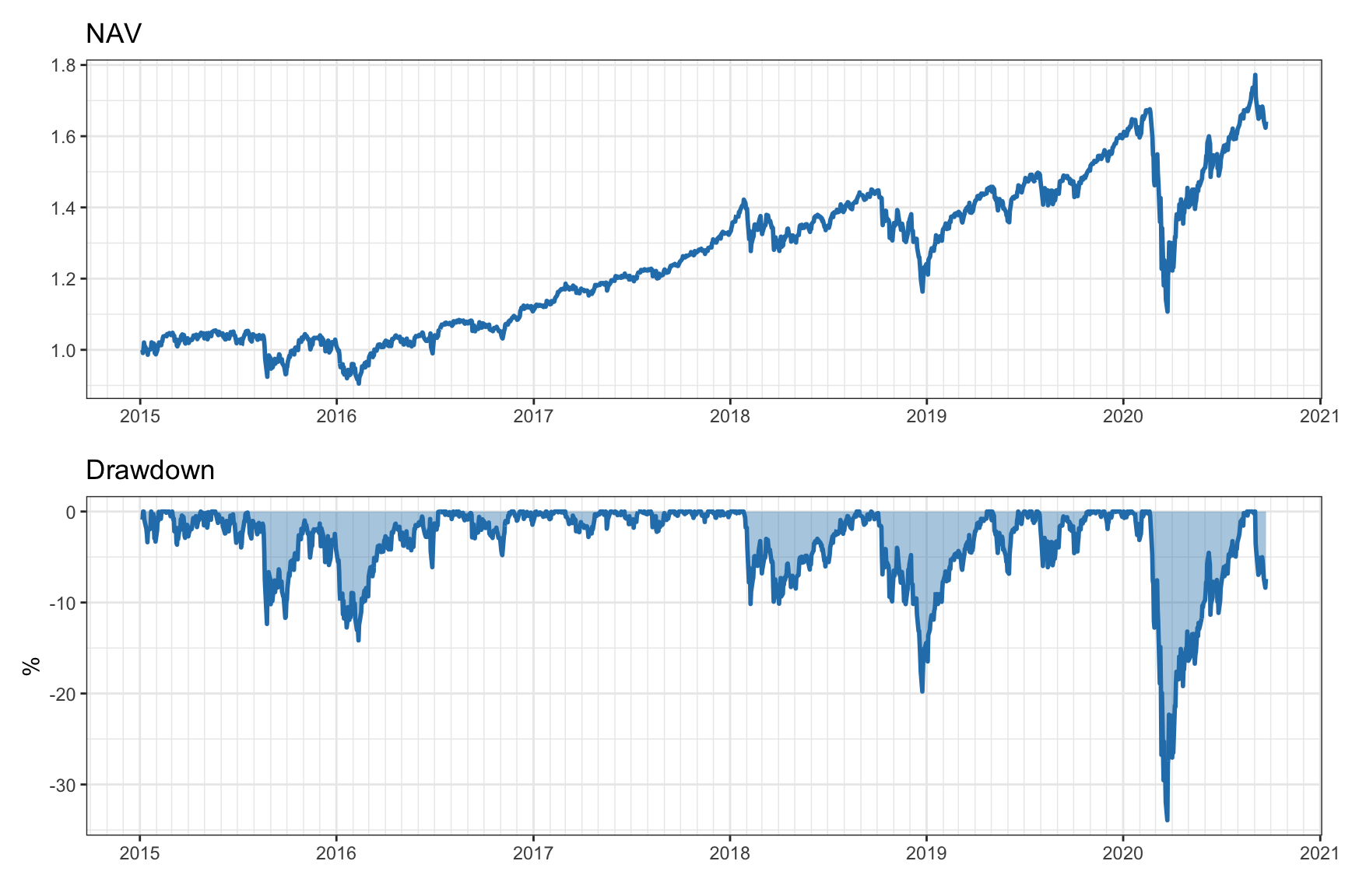
Figure 10.3: Illustration of NAV and corresponding drawdown.
Path Dependency
It is important to remark that the drawdown is a path-dependent measure. This means that it depends on the temporal order in which the returns happen. This is in sharp contrast to the previously considered measures, which are agnostic to the ordering of the returns.
For illustration purposes, Figure 10.4 shows the best and worst possible ordering of the returns corresponding to the original ordering in Figure 10.3. The difference is extreme: in the best case the drawdown reaches about 12.5%, whereas in the worst case it goes to virtually 100% (the original drawdown reached 34%).
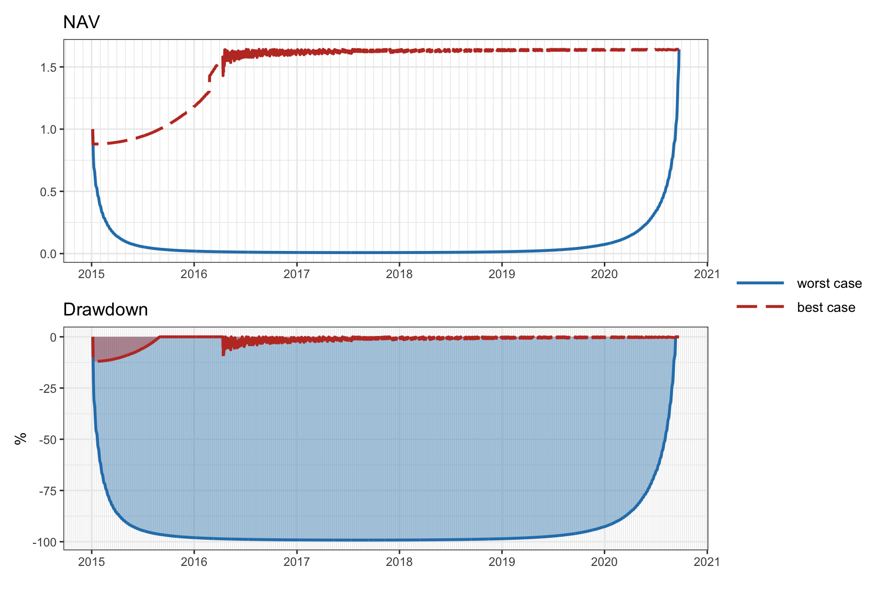
Figure 10.4: Effect of ordering of returns in the cumulative return and drawdown.
Single-Number Summarization
In practice, it is convenient to summarize the whole drawdown curve, which spans a period \(t=1,\ldots,T\), into a single number. This can be done in different ways:
- maximum drawdown (Max-DD): \[\textm{Max-DD} = \underset{1\le t\le T}{\textm{max}} D(t);\]
- average drawdown (Ave-DD): \[\textm{Ave-DD} = \frac{1}{T}\sum_{1\le t\le T} D(t);\]
- CVaR of drawdown (CVaR-DD) or conditional drawdown at risk (CDaR): \[\textm{CDaR}_{\alpha} = \E\left[D(t) \mid D(t)\geq\textm{VaR}_{\alpha}\right],\] where \(\textm{VaR}_{\alpha}\) is the value at risk of the drawdown \(D(t)\) with confidence level \(\alpha\).