11.7 General Nonconvex Formulations
Risk parity places risk management at the heart of the strategy by building risk-diversified portfolios while ignoring the expected return. It has been criticized precisely because it focuses on managing risk concentration rather than portfolio performance. However, the expected return can also be taken into account within the risk parity paradigm (Roncalli, 2013a). This is often referred to as the enhanced risk parity portfolio.
Section 11.6 was devoted to the vanilla formulation, that is, just with the portfolio constraints \(\bm{1}^\T\w=1\) and \(\w \ge \bm{0}\), which can be reformulated in convex form and optimally solved in order to obtain a portfolio satisfying the risk budgeting equations: \(w_i\left(\bSigma\w\right)_i = b_i \w^\T\bSigma\w,\;i=1,\ldots,N.\) However, in practice, portfolio managers always have additional constraints (e.g., turnover constraint, market-neutral constraint, maximum-position constraint) as listed in Section 6.2 and also additional objective functions such as the maximization of the expected return or minimization of the overall variance or volatility. In such realistic scenarios, unfortunately, the convex reformulations in Section 11.6 do not hold anymore and we need to resort to more complicated nonconvex formulations.
For the general case incorporating additional constraints and/or objective functions, the risk budgeting equations can only be approximately satisfied: \[w_i\left(\bSigma\w\right)_i \approx b_i \w^\T\bSigma\w, \qquad i=1,\ldots,N.\]
Since the risk budgeting constraints can only be satisfied approximately, we need to define a measure of the approximation error, but there is a multitude of possible choices, such as:
sum of squared relative risk-contribution errors: \[\sum_{i=1}^N \left(\frac{w_i\left(\bSigma\w\right)_i}{\w^\T\bSigma\w} - b_i\right)^2;\]
sum of squared risk-contribution errors: \[\sum_{i=1}^N \left(\frac{w_i\left(\bSigma\w\right)_i}{\sqrt{\w^\T\bSigma\w}} - b_i\sqrt{\w^\T\bSigma\w}\right)^2;\]
sum of squared volatility-scaled risk-contribution errors: \[\sum_{i=1}^N \left(w_i\left(\bSigma\w\right)_i - b_i \w^\T\bSigma\w\right)^2.\]
These three error definitions are the same up to a scaling factor; but in terms of numerical algorithms they show different convergence behaviors (notice that the gradients and Hessians are different). We recommend the use of the relative risk contributions since they are normalized by definition between 0 and 1, and do not suffer from numerical issues.
Another alternative to assess the concentration of a risk measure \(f\) is via the Herfindahl index (Roncalli, 2013b): \[ h(\w) \triangleq \sum_{i=1}^N \left(\frac{w_i \frac{\partial f}{\partial w_i}}{f(\w)}\right)^2, \] which satisfies \(1/N \leq h(\w) \leq 1\), with \(h(\w) = 1\) indicating that the risk is totally concentrated on a single asset and \(h(\w) = 1/N\) corresponding to the risk being equally distributed among all the assets. Hence, the smaller the Herfindahl index is, the more diversified the risk is. For the case of the volatility, it becomes \[ h(\w) = \sum_{i=1}^N \left(\frac{w_i(\bSigma\w)_i}{\w^\T\bSigma\w}\right)^2. \]
These expressions are all based on the \(\ell_2\)-norm; however, many alternative norms could be used instead, such as the \(\ell_1\)-norm, \(\ell_\infty\)-norm, or Huber’s robust penalty function. This leads to a multitude of possible portfolio formulations, some of which have been explored in the literature as described next.
11.7.1 Formulations
One of the earlier proposed formulations (Maillard et al., 2010) penalizes the differences between the volatility-scaled risk-contribution errors as \[\begin{equation} \begin{array}{ll} \underset{\w}{\textm{minimize}} & \begin{aligned}\sum_{i,j=1}^{N}\left(w_i\left(\bSigma\w\right)_i - w_j\left(\bSigma\w\right)_j\right)^{2}\end{aligned}\\ \textm{subject to} & \w \in \mathcal{W}, \end{array} \tag{11.9} \end{equation}\] which can obviously be generalized to include the risk budget profile \(\bm{b}=(b_1,\dots,b_N)\) simply by using the normalized terms \(w_i\left(\bSigma\w\right)_i/b_i\) instead of \(w_i\left(\bSigma\w\right)_i\).
To avoid the double-index summation in the formulation (11.9), the following alternative reformulation, with the additional dummy variable \(\theta\), reduces the number of terms from \(N^2\) to \(N\): \[\begin{equation} \begin{array}{ll} \underset{\w,\theta}{\textm{minimize}} & \begin{aligned}\sum_{i=1}^{N}\left(w_i\left(\bSigma\w\right)_i - \theta\right)^{2}\end{aligned}\\ \textm{subject to} & \w \in \mathcal{W}. \end{array} \tag{11.10} \end{equation}\] Note that the optimal \(\theta\) for a given \(\w\) is \(\theta = \frac{1}{N}\sum_{i=1}^{N} w_i\left(\bSigma\w\right)_i = \frac{1}{N}\w^\T\bSigma\w\).
The following formulation based on the relative risk-contribution errors was proposed in Bruder and Roncalli (2012): \[\begin{equation} \begin{array}{ll} \underset{\w}{\textm{minimize}} & \begin{aligned}\sum_{i=1}^N \left(\frac{w_i\left(\bSigma\w\right)_i}{\w^\T\bSigma\w} - b_i\right)^2\end{aligned}\\ \textm{subject to} & \w \in \mathcal{W}. \end{array} \tag{11.11} \end{equation}\]
Another alternative formulation is based on the minimization of the Herfindahl index (Roncalli, 2013b): \[\begin{equation} \begin{array}{ll} \underset{\w}{\textm{minimize}} & \begin{aligned}\sum_{i=1}^N \left(\frac{w_i(\bSigma\w)_i}{\w^\T\bSigma\w}\right)^2\end{aligned}\\ \textm{subject to} & \w \in \mathcal{W}, \end{array} \tag{11.12} \end{equation}\] which can be seen as a particular case of (11.11) with \(b_i=0\).
The formulations (11.9) and (11.10) are not recommended as they tend to suffer from numerical issues because the terms \(w_i\left(\bSigma\w\right)_i\) squared can become very small (in order to make them work, the covariance matrix \(\bSigma\) has to be artificially scaled up) (Mausser and Romanko, 2014). For this reason, the formulations (11.11) and (11.12), based on the normalized terms \(w_i\left(\bSigma\w\right)_i/(\w^\T\bSigma\w)\), are preferred for numerical stability.
Unified Formulation
A general risk parity formulation was proposed in Feng and Palomar (2015) as \[\begin{equation} \begin{array}{ll} \underset{\w}{\textm{minimize}} & \begin{aligned}\sum_{i=1}^N g_i(\w)^2 + \lambda F(\w)\end{aligned}\\ \textm{subject to} & \w \in \mathcal{W}, \end{array} \tag{11.13} \end{equation}\] where \(g_i(\w)\) denotes an arbitrary concentration error measure for the \(i\)th asset, for example, \[g_i(\w) = \frac{w_i\left(\bSigma\w\right)_i}{\w^\T\bSigma\w} - b_i,\] the function \(F(\w)\) denotes an arbitrary preference function, for example, \[F(\w) = -\w^\T\bmu + \frac{1}{2}\w^\T\bSigma\w,\] and \(\lambda\) is a trade-off hyper-parameter.
This formulation is general enough to embrace all the previously given formulations. The design of an effective algorithm is nevertheless nontrivial due to the nonconvexity of the term \(\sum_{i=1}^N g_i(\w)^2\).
Alternative Convex Formulation
An interesting convex reformulation as a second-order cone program (SOCP) was proposed in Mausser and Romanko (2014). Consider the formulation (11.10) after solving for \(\theta\): \[ \begin{array}{ll} \underset{\w}{\textm{minimize}} & \begin{aligned}\sum_{i=1}^{N}\left(\frac{1}{N}\w^\T\bSigma\w - w_i\left(\bSigma\w\right)_i\right)^{2}\end{aligned}\\ \textm{subject to} & \w \in \mathcal{W}. \end{array} \]
Instead of using the sum of the squares in the objective, we can focus on the worst-case performance: \[ \begin{array}{ll} \underset{\w}{\textm{minimize}} & \sqrt{\frac{1}{N}\w^\T\bSigma\w} - \underset{i}{\textm{min}} \; \sqrt{w_i\left(\bSigma\w\right)_i}\\ \textm{subject to} & \w \in \mathcal{W}. \end{array} \]
At this point, by defining the dummy variable \(\bm{z} = \bSigma\w\) and identifying the first term in the objective as the variable \(p\) and the second term as the variable \(t\), we can rewrite the problem as the following SOCP: \[ \begin{array}{ll} \underset{\w,\bm{z},p,t}{\textm{minimize}} & \begin{array}[t]{l} p - t \end{array}\\ \textm{subject to} & \begin{array}[t]{ll} \bm{z} = \bSigma\w, & \\ Np^2 \ge \w^\T\bSigma\w, &\\ t^2 \le w_i z_i, & \quad i=1,\dots,N,\\ p,t \ge 0, &\\ \bm{z} \ge \bm{0}, &\\ \w \in \mathcal{W}. \end{array} \end{array} \]
Note that the constraints \(t^2 \le w_i z_i\) are called hyperbolic constraints (also known as rotated second-order constraints) and can be written as the following second-order cone constraint (Lobo et al., 1998): \[ \left\|\left[\begin{array}{c} 2t\\ w_i - z_i \end{array}\right]\right\|_2 \le w_i + z_i. \] Similarly, constraints of the form \(w_i(\bSigma\w)_i \ge b_i \w^\T\bSigma\w\) can be rewritten as second-order cone constraints: \[ \left\|\left[\begin{array}{c} 2\sqrt{b_i}\bSigma^{1/2}\w\\ w_i - (\bSigma\w)_i \end{array}\right]\right\|_2 \le w_i + (\bSigma\w)_i. \]
Unfortunately, solving an SOCP has a higher complexity than solving a QP, as described in Section B.1, Appendix B. Therefore, as reported in Mausser and Romanko (2014), this formulation does not seem to be advantageous or competitive in terms of deriving fast practical algorithms.
Illustrative Example
Figure 11.10 shows the distribution of the portfolio weights and risk contribution for the \(1/N\) portfolio, the naive diagonal RPP, the vanilla convex RPP, and the general nonconvex RPP (in this case including an upper bound on the weights of 0.15 for illustration purposes).
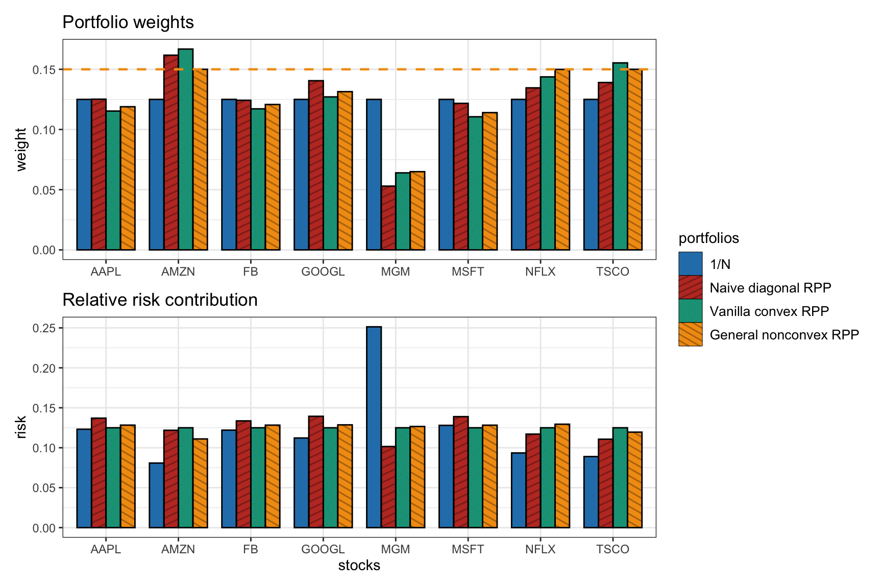
Figure 11.10: Portfolio allocation and risk contribution of general nonconvex RPP (with \(w_i \leq 0.15\)) compared to benchmarks (\(1/N\) portfolio, naive diagonal RPP, and vanilla convex RPP).
11.7.2 Algorithms
The previous nonconvex formulations can be solved with any general-purpose solver, cf. Mausser and Romanko (2014). As a more convenient and efficient alternative, we will now develop several practical iterative algorithms tailored to the problem formulations in (11.9)–(11.13) that produce a sequence of iterates \(\bm{w}^0, \bm{w}^1, \bm{w}^2,\dots\)
As the initial point of these iterative algorithms, one option is to use the solution provided by the vanilla convex formulation considered in Section 11.6 (effectively ignoring any additional constraints in \(\mathcal{W}\) and any additional objective function). However, some additional step is necessary to make sure that point is feasible taking into account all the constraints in \(\mathcal{W}\). A simpler alternative may be to simply use the \(1/N\) portfolio.
SCA Method
The SCA method can again be employed in this nonconvex case to develop efficient algorithms as proposed in Feng and Palomar (2015); for details on SCA, the reader is referred to Section B.8 in Appendix B.
Consider the objective function in the unified formulation (11.13): \[U(\w) = \sum_{i=1}^N g_i(\w)^2 + \lambda F(\w).\] One convenient way to convexify this function producing a quadratic function, which will be amenable for a QP solver, is to linearize the terms \(g_i(\w)\) around the current point \(\w^k\): \[ g_i(\w) \approx g_i(\w^k) + \nabla g_i(\w^k)^\T\left(\w - \w^k\right). \] This produces the following surrogate function for \(U(\w, \w^k)\): \[ \tilde{U}(\w, \w^k) = \sum_{i=1}^N \left(g_i(\w^k) + \nabla g_i(\w^k)^\T\left(\w - \w^k\right)\right)^2 + \lambda F(\w) + \frac{\tau}{2}\left\Vert \w-\w^{k}\right\Vert _{2}^{2}, \] where the last term is a regularizer to obtain a strongly convex function as required by SCA.
Finally, the approximated QP can be written (ignoring unnecessary constant terms) as \[\begin{equation} \begin{array}{ll} \underset{\w}{\textm{minimize}} & \frac{1}{2}\w^\T\bm{Q}^{k}\w+\w^\T\bm{q}^{k}+\lambda F(\w)\\ \textm{subject to} & \w \in \mathcal{W}, \end{array} \tag{11.14} \end{equation}\] where \[ \begin{aligned} \bm{Q}^k &\triangleq 2\left(\bm{J}^{k}\right)^\T\bm{J}^{k} + \tau\bm{I},\\ \bm{q}^k &\triangleq 2\left(\bm{J}^{k}\right)^\T\bm{g}^k - \bm{Q}^{k}\w^{k}, \end{aligned} \] and the vector of functions \(g_i\) and its Jacobian matrix at point \(\w^k\) are \[ \begin{aligned} \bm{g}^k &\triangleq \left[g_1(\w^k), \dots, g_N(\w^k)\right]^\T,\\ \bm{J}^k &\triangleq \left[\begin{array}{c} \nabla g_1(\w^k)^\T\\ \vdots\\ \nabla g_N(\w^k)^\T \end{array}\right]. \end{aligned} \]
This approximated QP can be solved directly with a QP solver or, depending on the constraints in \(\mathcal{W}\), even in closed form as developed in Feng and Palomar (2015).
The overall SCA method, termed Successive Convex optimization for RIsk Parity portfolio (SCRIP), is summarized in Algorithm 11.1. For additional details and more advanced algorithms, the reader is referred to (Feng and Palomar, 2015).
Algorithm 11.1: SCRIP to solve problem (11.13).
Choose initial point \(\w^0\in\mathcal{W}\) and sequence \(\{\gamma^k\}\);
Set \(k \gets 0\);
repeat
- Calculate risk concentration terms \(\bm{g}^k\) and Jacobian matrix \(\bm{J}^k\) for current point \(\w^{k}\);
- Solve approximated QP problem (11.14) and keep solution as \(\hat{\w}^{k+1}\);
- \(\w^{k+1} \gets \w^{k} + \gamma^k (\hat{\w}^{k+1} - \w^{k})\);
- \(k \gets k+1\);
until convergence;
Alternate Linearization Method
The alternate linearization method (ALM) was proposed in Bai et al. (2016) to solve the formulation in (11.10), whose objective is \[ F(\w,\theta) = \sum_{i=1}^{N}\left(w_i\left(\bSigma\w\right)_i - \theta\right)^{2} = \sum_{i=1}^{N}\left(\w^\T \bm{M}_i \w - \theta\right)^{2}, \] where matrix \(\bm{M}_i\) is defined to be of the same size as \(\bSigma\) containing the same \(i\)th row, \([\bm{M}_i]_{i,:} = [\bSigma]_{i,:}\), and zeros elsewhere.
The idea is to introduce an additional variable \(\bm{y}\) and then define \[ F(\w,\bm{y},\theta) = \sum_{i=1}^{N}\left(\w^\T \bm{M}_i \bm{y} - \theta\right)^{2}, \] subject to \(\bm{y}=\w\). Then, the algorithm optimizes \(\w\) and \(\bm{y}\) sequentially (and also \(\theta\)) by minimizing the following two QP approximations of \(F(\w,\bm{y},\theta)\): \[ \begin{aligned} Q^1(\w,\bm{y}^k,\theta) &\triangleq F(\w,\bm{y}^k,\theta) + \nabla_2 F(\bm{y}^k,\bm{y}^k,\theta)^\T (\w - \bm{y}^k) + \frac{1}{2\mu}\|\w - \bm{y}^k\|_2^2,\\ Q^2(\w^{k+1},\bm{y},\theta) &\triangleq F(\w^{k+1},\bm{y},\theta) + \nabla_1 F(\w^{k+1},\w^{k+1},\theta)^\T (\bm{y} - \w^{k+1}) + \frac{1}{2\mu}\|\bm{y} - \w^{k+1}\|_2^2, \end{aligned} \] where \(\mu\) is some chosen positive scalar and \[ \begin{aligned} \nabla_1 F(\w,\bm{y},\theta) &= 2\sum_{i=1}^{N}\left(\w^\T \bm{M}_i \bm{y} - \theta\right)\bm{M}_i \bm{y},\\ \nabla_2 F(\w,\bm{y},\theta) &= 2\sum_{i=1}^{N}\left(\w^\T \bm{M}_i \bm{y} - \theta\right)\bm{M}^\T_i \w. \end{aligned} \]
11.7.3 Numerical Experiments
To evaluate the algorithms empirically, we use a universe of \(N=200\) stocks from the S&P 500 and compare their convergence in terms of iterations as well as CPU time. We include the upper bound on the weights \(w_i \leq 0.008\) so that the formulation cannot be framed in the convex case considered in Section 11.6, and we use the simple initial point \(w_i = 1/N\) so that we can better observe the convergence.
Convergence for Formulation in (11.10)
We start with the nonconvex formulation in (11.10), which, in fact, is not recommended since the terms \(w_i\left(\bSigma\w\right)_i\) squared can become very small and lead to numerical issues; a practical heuristic is to scale up the covariance matrix \(\bSigma\) by some large number like \(10^4\) (Mausser and Romanko, 2014). For this reason, the formulations based on the normalized terms \(w_i\left(\bSigma\w\right)_i/(\w^\T\bSigma\w)\) are preferred for numerical stability, like in formulation (11.11).
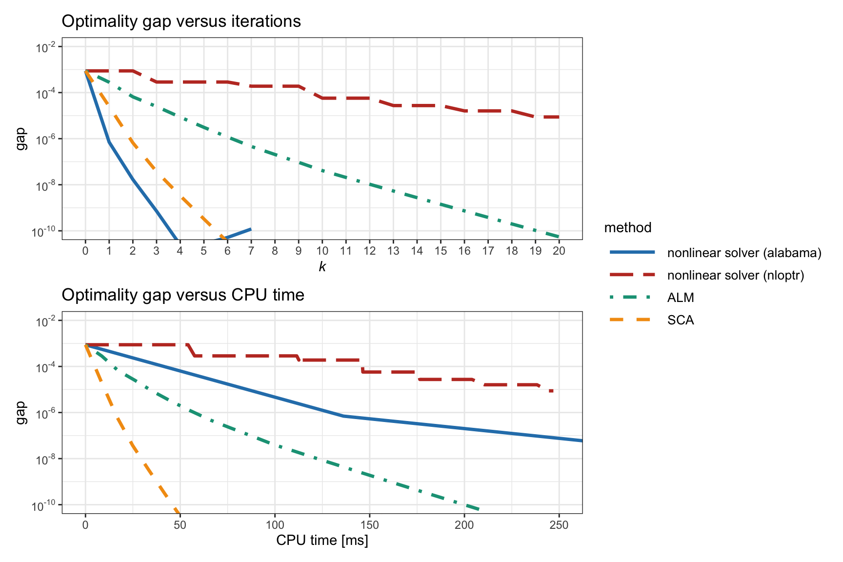
Figure 11.11: Convergence of different algorithms for the nonconvex RPP formulation (11.10).
Figure 11.11 shows the convergence of two general-purpose nonlinear solvers as well as the methods ALM and SCA. It is clear that the nonlinear solvers are less efficient as they do not exploit the problem structure. The SCA method is clearly the fastest to converge.
Convergence for Formulation in (11.11)
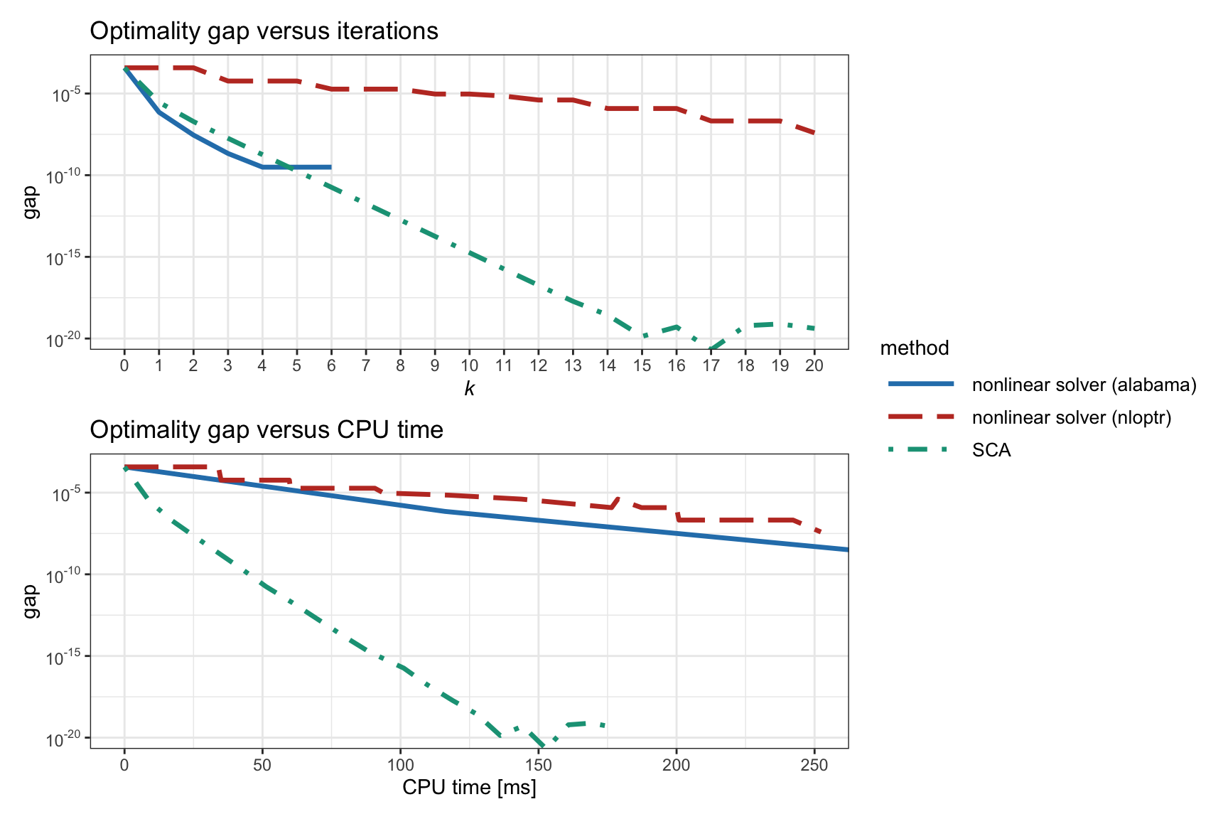
Figure 11.12: Convergence of different algorithms for the nonconvex RPP formulation (11.11) .
We now focus on the formulation in (11.11), which is preferred because the risk terms are normalized and do not suffer from numerical issues. Figure 11.12 shows the convergence of two general-purpose nonlinear solvers as well as the SCA method, which exhibits a much faster convergence.