3.2 Sample Estimators
In practice, the parameters of the i.i.d. model in (3.1), \((\bmu, \bSigma)\), are unknown and have to be estimated using historical data \(\bm{x}_1,\dots,\bm{x}_T\) containing \(T\) past observations. The simplest estimators are the sample mean, \[\begin{equation} \hat{\bmu} = \frac{1}{T}\sum_{t=1}^{T}\bm{x}_{t}, \tag{3.2} \end{equation}\] and the sample covariance matrix, \[\begin{equation} \hat{\bSigma} = \frac{1}{T-1}\sum_{t=1}^{T}(\bm{x}_t - \hat{\bmu})(\bm{x}_t - \hat{\bmu})^\T, \tag{3.3} \end{equation}\] where the “hat” notation “\(\;\hat{\;}\;\)” denotes estimation.
One important property is that these estimators are unbiased, namely, \[ \E\left[\hat{\bmu}\right] = \bmu, \qquad \E\big[\hat{\bSigma}\big] = \bSigma. \] In words, the random estimates \(\hat{\bmu}\) and \(\hat{\bSigma}\) are centered around the true values. In fact, the factor of \(1/(T - 1)\) in the sample covariance matrix is precisely chosen so that the estimator is unbiased; if, instead, the more natural factor \(1/T\) is used, then the estimator is biased: \(\E\big[\hat{\bSigma}\big] = \left(1 - \frac{1}{T}\right)\bSigma.\)
Another important property is that these estimators are consistent, that is, from the law of large numbers (T. W. Anderson, 2003; Papoulis, 1991) it follows that \[ \lim_{T\rightarrow\infty} \hat{\bmu} = \bmu, \qquad \lim_{T\rightarrow\infty} \hat{\bSigma} = \bSigma. \]
In words, the sample estimates converge to the true quantities as the number of observations \(T\) grows. Figure 3.2 shows how the estimation error indeed goes to zero as \(T\) grows for synthetic Gaussian data of dimension \(N=100\) (in particular, the normalized error is used, defined as \(100\times\|\hat{\bmu} - \bmu\|/\|\bmu\|\) for the case of the sample mean, and similarly for the sample covariance matrix).
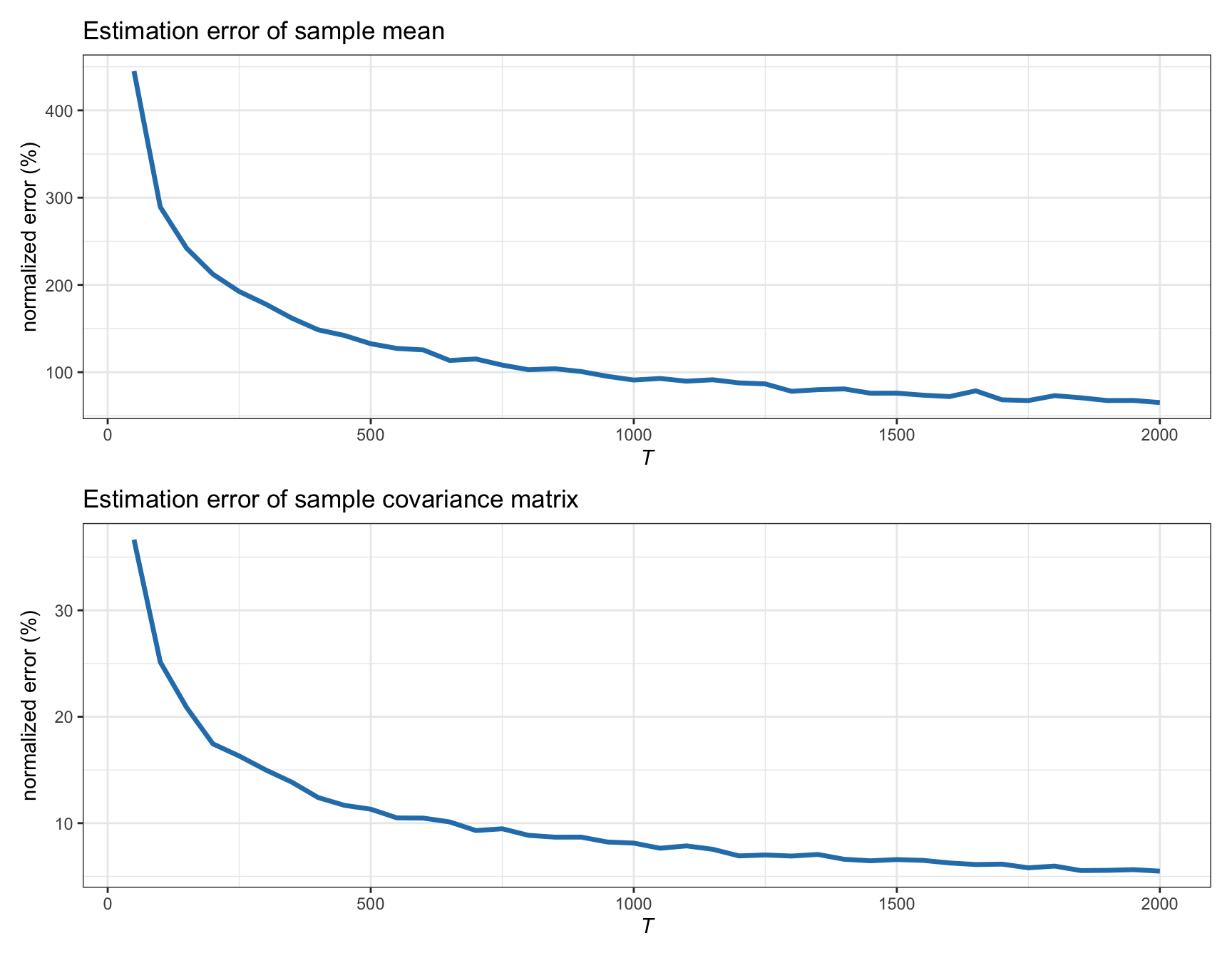
Figure 3.2: Estimation error of sample estimators vs. number of observations (for Gaussian data with \(N=100\)).
These sample estimators \(\hat{\bmu}\) and \(\hat{\bSigma}\) are easy to understand, simple to implement, and cheap in terms of computational cost. However, they are only good estimators for a large number of observations \(T\); otherwise, the estimation error becomes unacceptable. In particular, the sample mean is a very inefficient estimator, producing very noisy estimates (Chopra and Ziemba, 1993; Meucci, 2005). This can be observed in Figure 3.2, where the normalized error of \(\hat{\bmu}\) for \(N=100\) and \(T=500\) is over 100%, which means that the error is as large as the true \(\bmu\). In practice, however, there are two main reasons why \(T\) cannot be chosen large enough to produce good estimations:
Lack of available historical data: For example, if we use use daily stock data (i.e., 252 observations per year) and the universe size is, say, \(N=500\), then a popular rule of thumb suggests that we should use \(T \approx 10\times N\) observations, which means 20 years of data. Generally speaking, 20 years of data are rarely available for the whole universe of assets.
Lack of stationarity: Even if we had available all the historical data we wanted, because financial data is not stationary over long periods of time, it does not make much sense to use such data: the market behavior and dynamics 20 years ago are too different from the current ones (cf. Chapter 2).
As a consequence, in a practical setting, the amount of data that can be used is very limited. But then, the estimates \(\hat{\bmu}\) and \(\hat{\bSigma}\) will be very noisy, particularly the sample mean. This is, in fact, the “Achilles’ heel” of portfolio optimization: \(\hat{\bmu}\) and \(\hat{\bSigma}\) will inevitably contain estimation noise which will lead to erratic portfolio designs. This is why Markowitz’s portfolio has not been fully embraced by practitioners.
In the rest of this chapter, we will get a deeper perspective on why sample estimators perform so poorly with financial data and, then, we will explore a number of different ways to improve them.