13.2 Sparse Regression
A vector is sparse if it has many elements equal to zero. Sparsity is a very important property in a wide variety of problems where proper control of the sparsity level is desired (Elad, 2010).
The cardinality of a vector \(\bm{x}\in\R^N\), denoted by \(\textm{card}(\bm{x})\), refers to the number of nonzero elements: \[ \textm{card}(\bm{x}) \triangleq \sum_{i=1}^N 1\{x_i \neq 0\}, \] where \(1\{\cdot\}\) denotes the indicator function. It is often written as the \(\ell_0\)-pseudo-norm \(\|\bm{x}\|_0\), which is not a norm (in fact, it is not even convex).
13.2.1 Problem Formulation
Sparse regression refers to a regression problem with the additional requirement that the solution has to be sparse. Some common formulations of sparse regression includes:
Regularized sparse least squares (LS): \[ \begin{array}{ll} \underset{\bm{x}}{\textm{minimize}} & \left\Vert \bm{A}\bm{x} - \bm{b} \right\Vert_2^2 + \lambda \|\bm{x}\|_0, \end{array} \] where the parameter \(\lambda\) can be chosen to enforce more or less sparsity in the solution.
Constrained sparse LS: \[ \begin{array}{ll} \underset{\bm{x}}{\textm{minimize}} & \left\Vert \bm{A}\bm{x} - \bm{b} \right\Vert_2^2\\ \textm{subject to} & \|\bm{x}\|_0 \leq k, \end{array} \] where \(k\) is a parameter to control the sparsity level.
Sparse underdetermined system of linear equations: \[ \begin{array}{ll} \underset{\bm{x}}{\textm{minimize}} & \|\bm{x}\|_0\\ \textm{subject to} & \bm{A}\bm{x} = \bm{b}, \end{array} \] where the system of linear equations \(\bm{A}\bm{x} = \bm{b}\) is underdetermined (so that it has an infinite number of solutions).
Unfortunately, the cardinality operator is noncontinuous, nondifferentiable, and nonconvex, which means that developing practical algorithms under sparsity is not trivial. As a matter of fact, this has been a well-researched topic for decades and mature approximate methods are currently available, as described next.
13.2.2 Methods for Sparse Regression
The most common approach to deal with the cardinality operator is to approximate it with a more convenient form for optimization methods. Figure 13.3 shows the following two approximations (along with the indicator function):
\(\ell_1\)-norm approximation: \(\|\bm{x}\|_0\) is simply approximated by \(\|\bm{x}\|_1\). In the univariate case, it means that the indicator function \(1\{t \neq 0\}\) is approximated by the absolute value \(|t|\).
Concave approximation: \(\|\bm{x}\|_0\) is better approximated by a concave function (rendering the sparse regression problem nonconvex). In the univariate case, it means that the indicator function \(1\{t \neq 0\}\) is approximated by a concave function, such as the log-function \(\textm{log}(1+t/\varepsilon)\), where \(\varepsilon\) is a parameter controlling the accuracy of the approximation, although many other concave approximation have been proposed (Candès et al., 2008).
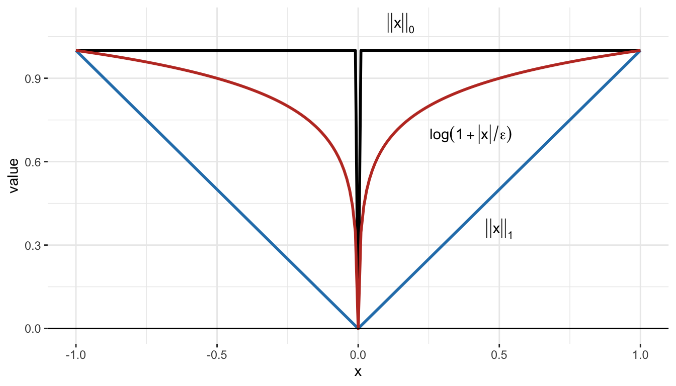
Figure 13.3: Indicator function and approximations.
\(\ell_1\)-Norm Approximation
The most popular algorithm for sparse regression is undoubtedly the LASSO (least absolute shrinkage and selection operator) (Tibshirani, 1996), which solves the following convex quadratic problem based on the \(\ell_1\)-norm approximation: \[ \begin{array}{ll} \underset{\bm{x}}{\textm{minimize}} & \left\Vert \bm{A}\bm{x} - \bm{b} \right\Vert_2^2\\ \textm{subject to} & \|\bm{x}\|_1 \leq t, \end{array} \] where \(t\) is a parameter to control the sparsity level.
Another popular method for sparse regression is the elastic net (Zou and Hastie, 2005), which overcomes some of the limitations of the LASSO. In particular, if groups of variables are highly correlated, the LASSO tends to select one variable from a group and ignore the others. The elastic net is a regularized regression method that linearly combines the \(\ell_1\) and \(\ell_2\) penalties of the LASSO and ridge methods.
It is worth noting that nonnegativity constraints alone can also induce sparsity in the solution (Meinshausen, 2013).
Similarly, the sparse resolution of an underdetermined system of linear equations can be recovered in practice, under some technical conditions, as a linear program (Candès and Tao, 2005; Donoho, 2006): \[ \begin{array}{ll} \underset{\bm{x}}{\textm{minimize}} & \|\bm{x}\|_1\\ \textm{subject to} & \bm{A}\bm{x} = \bm{b}. \end{array} \]
Concave Approximation
In some cases, the \(\ell_1\)-norm approximation is not good enough and one needs to resort to a more refined concave approximation (as illustrated in Figure 13.3): \[ \|\bm{x}\|_0 \approx \sum_{i=1}^N \phi(|x_i|), \] where \(\phi(\cdot)\) is an appropriate concave function, such as the popular log-function \[ \phi(t) = \textm{log}(1+t/\varepsilon). \] Alternative concave approximations can be used (Candès et al., 2008), such as the arc-tangent function or the \(\ell_p\)-norm for \(0<p<1\).
However, a concave approximation leads to a nonconvex problem formulation, such as \[ \begin{array}{ll} \underset{\bm{x}}{\textm{minimize}} & \begin{aligned}[t] \left\Vert \bm{A}\bm{x} - \bm{b} \right\Vert_2^2 + \lambda \sum_{i=1}^N \textm{log}\left(1 + \frac{|x_i|}{\varepsilon}\right) \end{aligned}. \end{array} \] Fortunately, we can use the majorization–minimization framework to derive iterative methods to solve problems with concave approximations of the cardinality, as explored next. Other families of algorithms have also been successfully employed such as iteratively reweighted least squares (IRLS) minimization (Daubechies et al., 2010).
13.2.3 Preliminaries on MM
The majorization–minimization (MM) method (or framework) approximates a difficult optimization problem by a sequence of simpler approximated problems. We now give a concise description. For details, the reader is referred to Section B.7 in Appendix B, as well as the concise tutorial in Hunter and Lange (2004), the long tutorial with applications in Y. Sun et al. (2017), and the convergence analysis in Razaviyayn et al. (2013).
Suppose the following (difficult) problem is to be solved: \[ \begin{array}{ll} \underset{\bm{x}}{\textm{minimize}} & f(\bm{x})\\ \textm{subject to} & \bm{x} \in \mathcal{X}, \end{array} \] where \(f(\cdot)\) is the (possibly nonconvex) objective function and \(\mathcal{X}\) is a (possibly nonconvex) set. Instead of attempting to directly obtain a solution \(\bm{x}^\star\) (either a local or global solution), the MM method will produce a sequence of iterates \(\bm{x}^0, \bm{x}^1, \bm{x}^2,\dots\) that will converge to \(\bm{x}^\star\).
More specifically, at iteration \(k\), MM approximates the objective function \(f(\bm{x})\) by a surrogate function around the current point \(\bm{x}^k\) (essentially, a tangent upper bound), denoted by \(u\left(\bm{x};\bm{x}^k\right)\), leading to the sequence of (simpler) problems: \[ \bm{x}^{k+1}=\textm{arg}\underset{\bm{x}\in\mathcal{X}}{\textm{min}}\;u\left(\bm{x};\bm{x}^k\right), \qquad k=0,1,2,\dots \]
In order to guarantee convergence of the iterates, the surrogate function \(u\left(\bm{x};\bm{x}^k\right)\) has to satisfy the following technical conditions (Razaviyayn et al., 2013; Y. Sun et al., 2017):
- upper bound property: \(u\left(\bm{x};\bm{x}^k\right) \geq f\left(\bm{x}\right)\);
- touching property: \(u\left(\bm{x}^k;\bm{x}^k\right) = f\left(\bm{x}^k\right)\); and
- tangent property: \(u\left(\bm{x};\bm{x}^k\right)\) must be differentiable with \(\nabla u\left(\bm{x};\bm{x}^k\right) = \nabla f\left(\bm{x}\right)\).
The surrogate function \(u\left(\bm{x};\bm{x}^k\right)\) is also referred to as a majorizer because it is an upper bound of the original function. The fact that, at each iteration, first the majorizer is constructed and then it is minimized gives the name majorization–minimization to the method.
13.2.4 Iterative Reweighted \(\ell_1\)-Norm Minimization
We now employ the MM framework to derive an iterative algorithm to solve sparse regression problems. For illustration purposes, we will focus on the following formulation with a concave approximation of the cardinality operator: \[\begin{equation} \begin{array}{ll} \underset{\bm{x}}{\textm{minimize}} & \begin{aligned}[t] \sum_{i=1}^N \textm{log}\left(1 + \frac{|x_i|}{\varepsilon}\right) \end{aligned}\\ \textm{subject to} & \bm{A}\bm{x} = \bm{b}. \end{array} \tag{13.1} \end{equation}\] Recall that many other concave functions can be used similarly (Candès et al., 2008).
In order to use MM, we need a key component: a majorizer of the concave function \(\textm{log}(1+t/\varepsilon)\), which means that it has to be an upper-bound tangent on the point of interest.
Lemma 13.1 (Majorizer of the log function) The concave function \(\phi(t) = \log(1+t/\varepsilon)\) is majorized at \(t=t_0\) by its linearization: \[ \phi(t) \le \phi(t_0) + \phi(t_0)'(t-t_0) = \phi(t_0) + \frac{1}{\varepsilon + t_0}(t-t_0). \]
According to Lemma 13.1, the term \(\textm{log}\left(1 + |x_i|/\varepsilon\right)\) is majorized at \(x_{i}^{k}\) (up to an irrelevant constant) by \(\alpha_i^k\left|x_{i}\right|\) with weight \(\alpha_i^k = 1/(\varepsilon + |x_{i}^k|)\).
Concluding, we can solve the nonconvex problem (13.1) by solving the following sequence of convex problems (Candès et al., 2008), for \(k=0,1,2,\dots\): \[\begin{equation} \begin{array}{ll} \underset{\bm{x}}{\textm{minimize}} & \begin{aligned}[t] \sum_{i=1}^N \alpha_i^k|x_i| \end{aligned}\\ \textm{subject to} & \bm{A}\bm{x} = \bm{b}, \end{array} \tag{13.2} \end{equation}\] where the objective function is a weighted \(\ell_1\)-norm with weights \(\alpha_i^k = 1/(\varepsilon + |x_{i}^k|)\). That is, the concave approximation of the sparse regression in (13.1) has been effectively solved by a sequence of iterative reweighted \(\ell_1\)-norm minimization problems as in (13.2) (Candès et al., 2008).