2.4 Temporal Structure
Are the returns i.i.d. or do they show some temporal structure? This is a key question in finance because it determines the problem of forecasting the returns or prices. In fact, this has been a highly debated topic in economics for decades.
The efficient-market hypothesis (EMH) states that share prices reflect all information and consistent “alpha”8 generation is impossible (Fama, 1970). Accordingly, stocks always trade at their fair value on exchanges, making it impossible for investors to purchase undervalued stocks or sell stocks for inflated prices. Therefore, it should be impossible to outperform the overall market through expert stock selection or market timing, and the only way an investor can obtain higher returns is by purchasing riskier investments.
Although it is a cornerstone of modern financial theory, the EMH is highly controversial and often disputed (Shiller, 1981). Believers argue it is pointless to search for undervalued stocks or to try to predict trends in the market through either fundamental or technical analysis. Theoretically, neither technical nor fundamental analysis can produce risk-adjusted excess returns (i.e., “alpha”) consistently, and only insider information can result in outsized risk-adjusted returns. Although academics present a substantial body of evidence in support of it, there is an equal amount of dissent as well. For example, the fundamental-based investor Warren Buffett or the hedge fund Renaissance Technologies’ Medallion Fund have consistently beaten the market over long periods, which by definition is impossible according to the EMH.
Proponents of the EMH conclude that, because of the randomness of the market, investors could do better by investing in a low-cost, passive portfolio. On the other hand, opponents insist on the possibility of designing portfolios that can beat the market.
Some accessible textbooks that cover temporal analysis include Tsay (2010), Cowpertwait and Metcalfe (2009), and Ruppert and Matteson (2015).
2.4.1 Linear Structure in Returns
The autocorrelation function (ACF) and partial autocorrelation function (PACF) are heavily used in time series analysis and forecasting. They measure the linear structure or dependency along the temporal domain, which, according to the EMH, should be insignificant (Ding and Granger, 1996). The autocorrelation is simply the correlation between the signal at a time and some previous time, whereas the partial autocorrelation eliminates the effect of the signal in between those two time instances.
Figure 2.17 indicates that the S&P 500 index exhibits almost no significant autocorrelation that can be exploited by models for forecasting (lags other than zero are basically within the statistical insignificant level). Figure 2.18 similarly illustrates that there is no significant autocorrelation to be exploited in Bitcoin (hourly returns similarly show no autocorrelations).
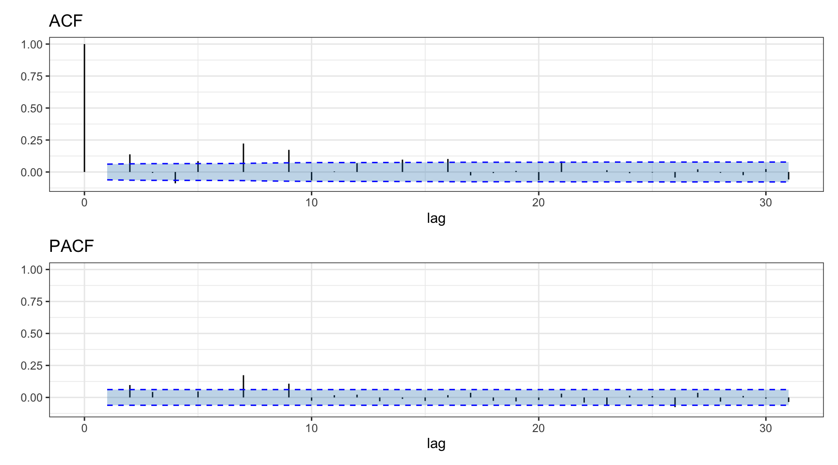
Figure 2.17: Autocorrelation of S&P 500 daily log-returns.
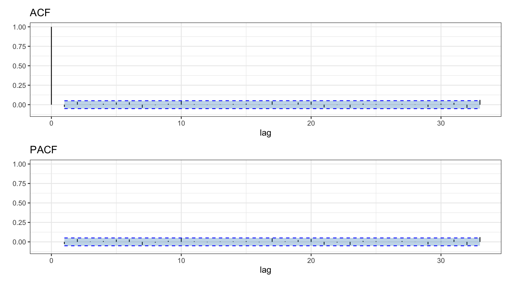
Figure 2.18: Autocorrelation of Bitcoin daily log-returns.
2.4.2 Nonlinear Structure in Returns
From the previous absence of significant autocorrelations, one may be tempted to conclude that there is no temporal structure to be exploited. However, that would be a wrong conclusion. A visual inspection of the returns suffices to see that clearly some structure is present in the volatility envelope of the signal (Ding and Granger, 1996), which measures the time-varying standard deviation of the signal along the time domain.
Figure 2.19 shows S&P 500 log-returns together with the volatility envelope, illustrating the phenomenon of the so-called volatility clustering. Clearly the volatility envelope changes slowly and can be easily forecast, as already pointed out in the 1990s (Ding and Granger, 1996). Figure 2.20 shows Bitcoin log-returns together with the volatility envelope, also exhibiting volatility clustering.
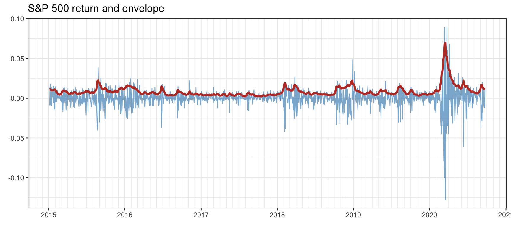
Figure 2.19: Volatility clustering in S&P 500.
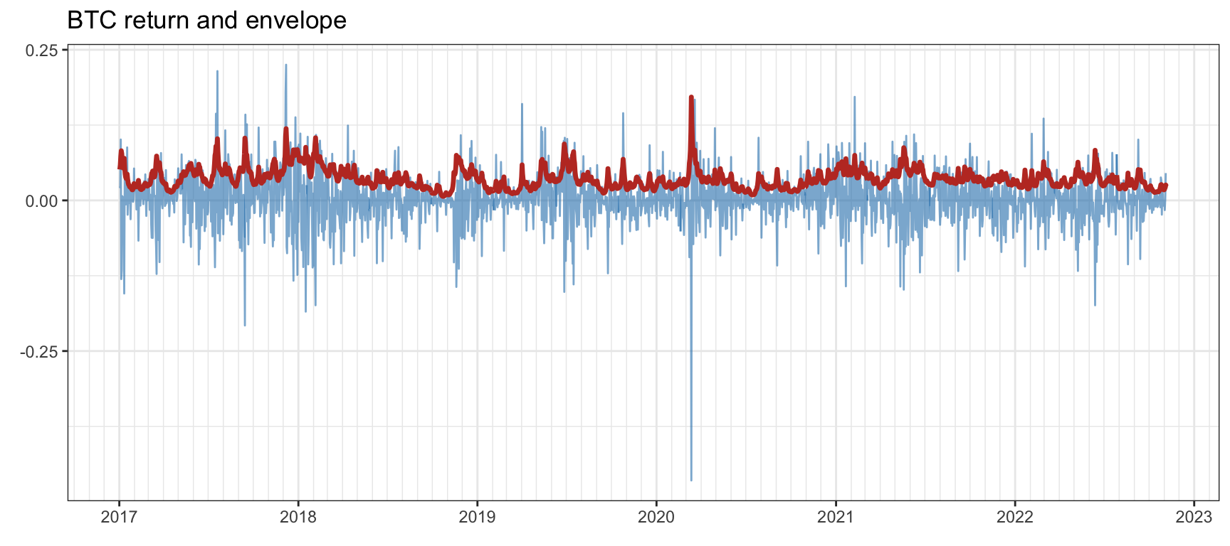
Figure 2.20: Volatility clustering in Bitcoin.
But how can it be that the returns show no significant autocorrelations but clearly there is some temporal structure?
The answer lies in the fact that autocorrelation measures only the linear dependency. Nonlinear dependencies are more elusive to detect. In fact, machine learning is a potential tool to try to identify such nonlinear dependencies (López de Prado, 2018a).
Since the envelope is basically a smooth version of the absolute value of the signal, one could calculate instead the autocorrelation of the absolute values of the returns. Figure 2.21 shows very significant autocorrelation values for the absolute values of the S&P 500 log-returns. Similarly, Figure 2.22 shows significant autocorrelation values for the absolute values of Bitcoin log-returns (albeit not as significant as in the case of the S&P 500).
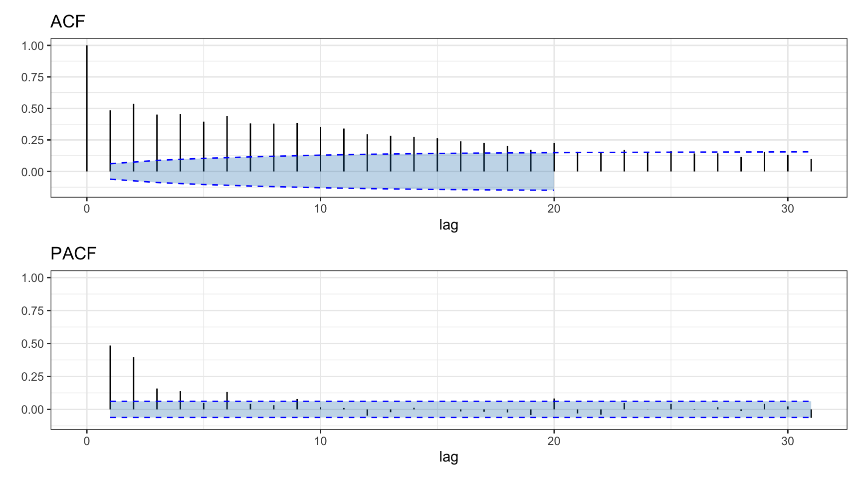
Figure 2.21: Autocorrelation of absolute value of S&P 500 daily log-returns.
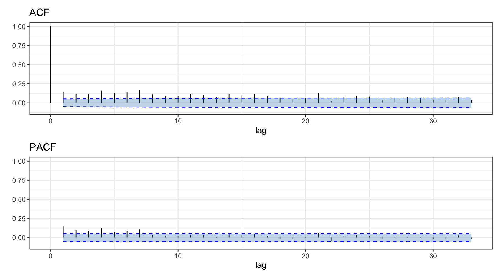
Figure 2.22: Autocorrelation of absolute value of Bitcoin daily log-returns.
It may be useful to factor out the volatility envelope from the returns (i.e., dividing the returns by the volatility) so as to obtain a time series without volatility clustering, termed standardized returns. Figures 2.23 and 2.24 illustrate such standardized returns for the S&P 500 and Bitcoin.
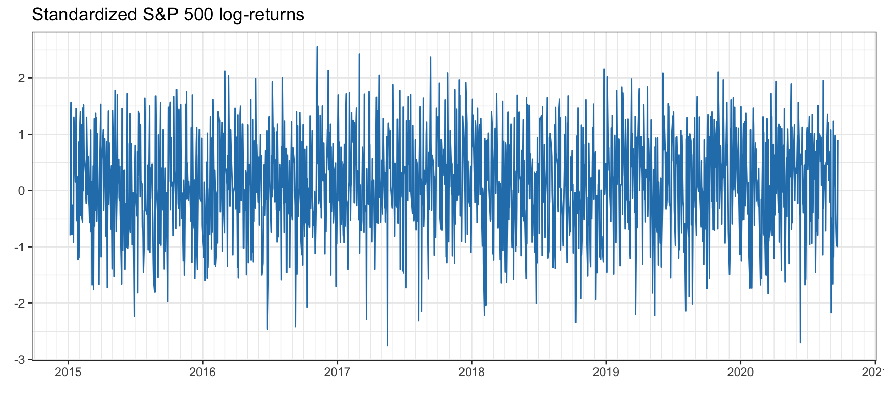
Figure 2.23: Standardized S&P 500 log-returns after factoring out the volatility envelope.
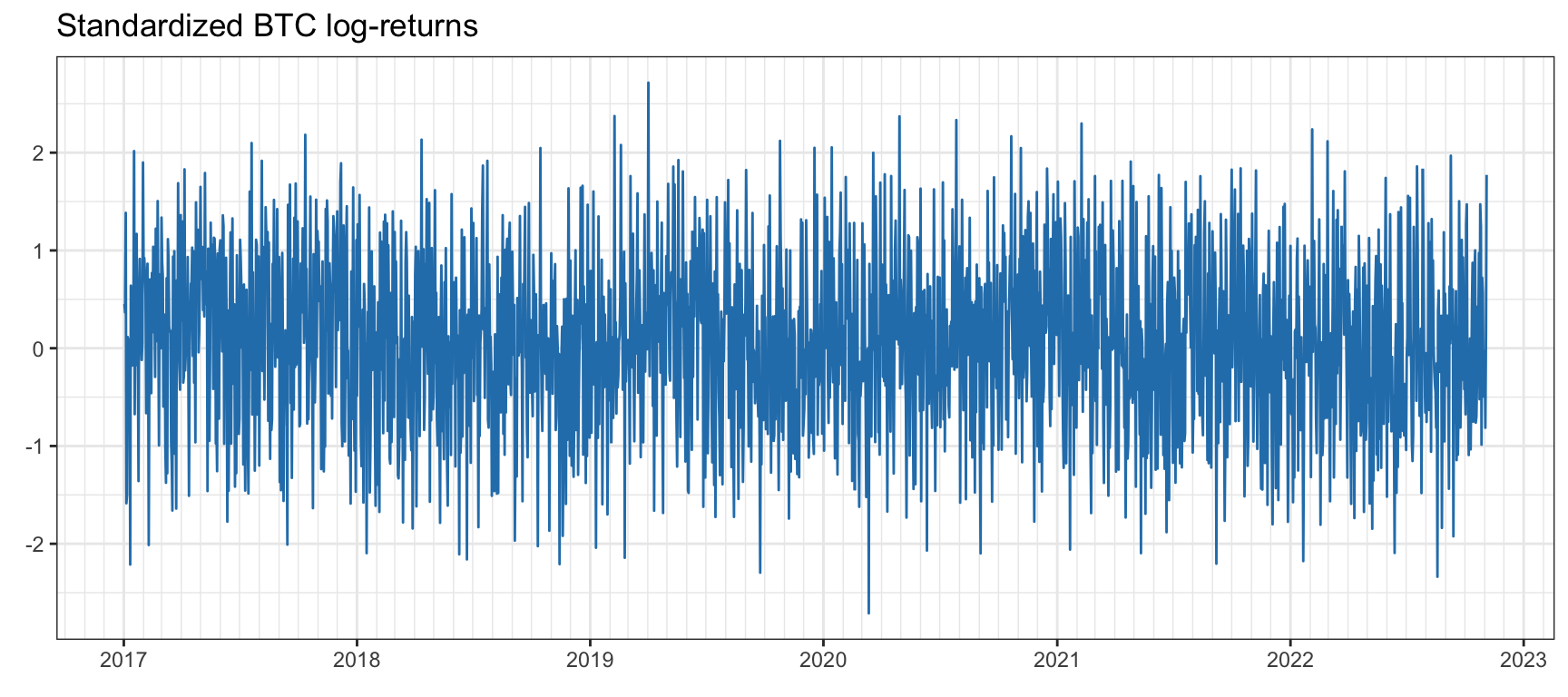
Figure 2.24: Standardized Bitcoin log-returns after factoring out the volatility envelope.
References
In finance, the term “alpha” is commonly used to denote a signal or information that results in the outperformance of profits compared to a benchmark.↩︎