15.1 Mean Reversion
Mean reversion is a property of a time series that means that there is a long-term average value around which the series may fluctuate over time but eventually will revert back to (Chan, 2013; Ehrman, 2006; Vidyamurthy, 2004). This property plays a crucial role in pairs trading, where the mean-reverting time series is artificially constructed by combining two (or more) assets. The mean reversion allows the trader to buy at a low price with the expectation that the price will return to the long-term mean over time. When the price reverts back to its historical average, the trader will close the position to realize a profit. Of course, this relies on the assumption that the historical relationship between the assets will persist in the future, which carries some risk; careful monitoring is key.
More generally, there are two types of mean reversion that trading strategies commonly exploit (Chan, 2013):
Longitudinal or time series mean reversion: This occurs when mean reversion takes place along the time axis, and there is a long-term average value. The deviation happens at one point in time in one direction and at another point in time in the opposite direction.
Cross-sectional mean reversion: This type of mean reversion occurs along the asset axis, and there is an average value across assets. Some assets deviate in one direction, while others deviate in the opposite direction (Fabozzi et al., 2010).
Stationarity is a property related to mean reversion, but different. Stationarity refers to the property that the statistics of a time series remain fixed over time. In that sense, a stationary time series can be considered mean reverting (Vidyamurthy, 2004), but not the other way around.
Unit-root stationarity is a specific type of stationarity (Tsay, 2010, 2013). It refers to modeling the time series with an autoregressive (AR) model with no unit roots (this is related to an Ornstein–Uhlenbeck process in continuous time). A time series with a unit root is not stationary and tends to diverge over time. A notable example of unit-root nonstationarity is the random walk model commonly employed for log-prices (see Chapter 3): \[ y_{t} = \mu + y_{t-1} + \epsilon_t, \] where \(y_{t}\) denotes the log-price at period \(t\), \(\mu\) is the drift, and \(\epsilon_t\) is the residual. Figure 15.1 shows an example of a time series with a unit root that does not return to the mean in a controlled way.61 On the other hand, in the absence of a unit root, the time series will not diverge and will eventually return to the mean; an example is the AR model of order 1 (AR(1)): \[ y_{t} = \mu + \rho\,y_{t-1} + \epsilon_t, \] with \(|\rho|<1\). Figure 15.2 illustrates an AR(1) time series with no unit root (\(\rho=0.2\)) and \(\mu=0\), which reverts to the mean in a controlled way.
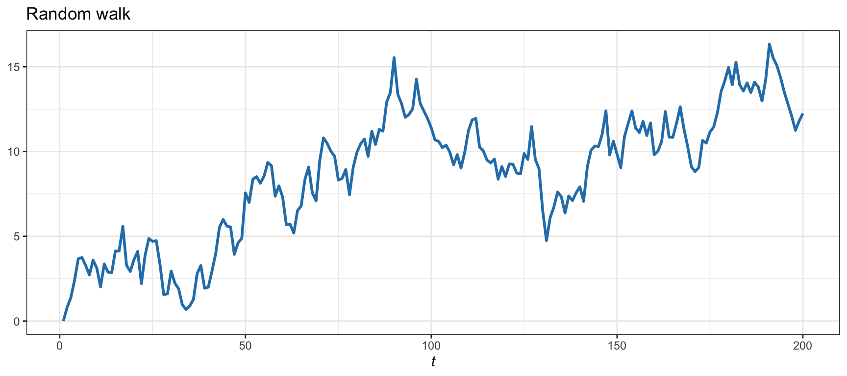
Figure 15.1: Example of a random walk (nonstationary time series with unit root).
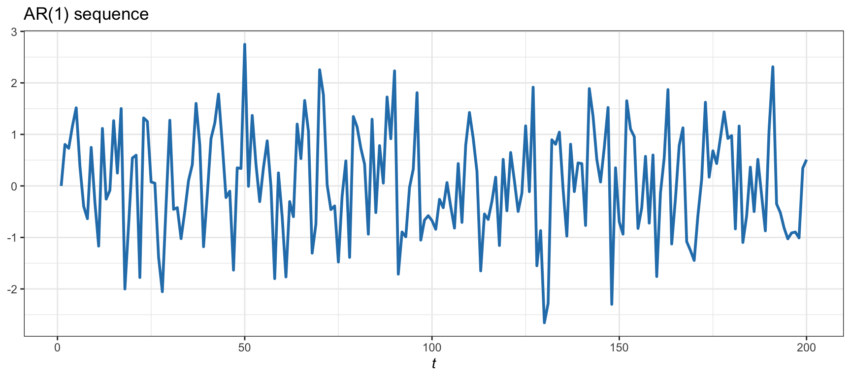
Figure 15.2: Example of a unit-root stationary AR(1) sequence.
Even though mean reversion and unit-root stationarity are not equivalent concepts, from a practical standpoint unit-root stationarity is a convenient proxy for mean reversion (Tsay, 2010, 2013). In fact, testing for unit-root stationarity is the de facto approach for determining mean reversion in practice.
Differencing is an operation commonly used to obtain stationarity (Tsay, 2010, 2013). It refers to taking differences between consecutive samples of a time series \(y_1, y_2, y_3, \dots\) to produce \(\Delta y_t = y_t - y_{t-1}\). The importance of this operation is that a nonstationary time series, such as a random walk, may become stationary after differencing. This is precisely the case when differencing the log-prices of an asset to obtain the log-returns (see Chapter 3 for details); we then say that log-prices are integrated of order 1 (higher-order differencing can also be considered).
References
Mathematically, it can be shown that a random walk in one dimension and even in two dimensions (e.g., a drunken man walking on a surface) will eventually return to the starting point. Interestingly, this property does not hold in three dimensions (e.g., a drunken bird flying).↩︎