5.1 Graphs
Graphs have become a fundamental and ubiquitous mathematical tool for modeling data in a variety of application domains and for understanding the structure of large networks that generate data (Kolaczyk, 2009; Lauritzen, 1996). By abstracting the data as graphs, we can better capture the geometry of data and visualize high-dimensional data. Some iconic examples of graphs, illustrated in Figure 5.1, include the following:
Social media graphs: These model the behavioral similarity or influence between individuals, with the data consisting of online activities such as tagging, liking, purchasing, and so on.
Brain activity graphs: These represent the correlation among sensors examining the brain, with the data being the measured brain activity known as fMRI (functional magnetic resonance imaging).
Financial stock graphs: These capture the interdependencies among financial companies in stock markets, with the data consisting of measured economic quantities such as stock prices, volumes, and so on.
Financial currency graphs: These summarize the interdependencies among currencies in foreign exchange markets, with the data comprising measured economic quantities like spot prices, volumes, and so on.
Financial cryptocurrency graphs: Similarly to currency graphs, these model the interdependencies among cryptocurrencies in crypto markets.
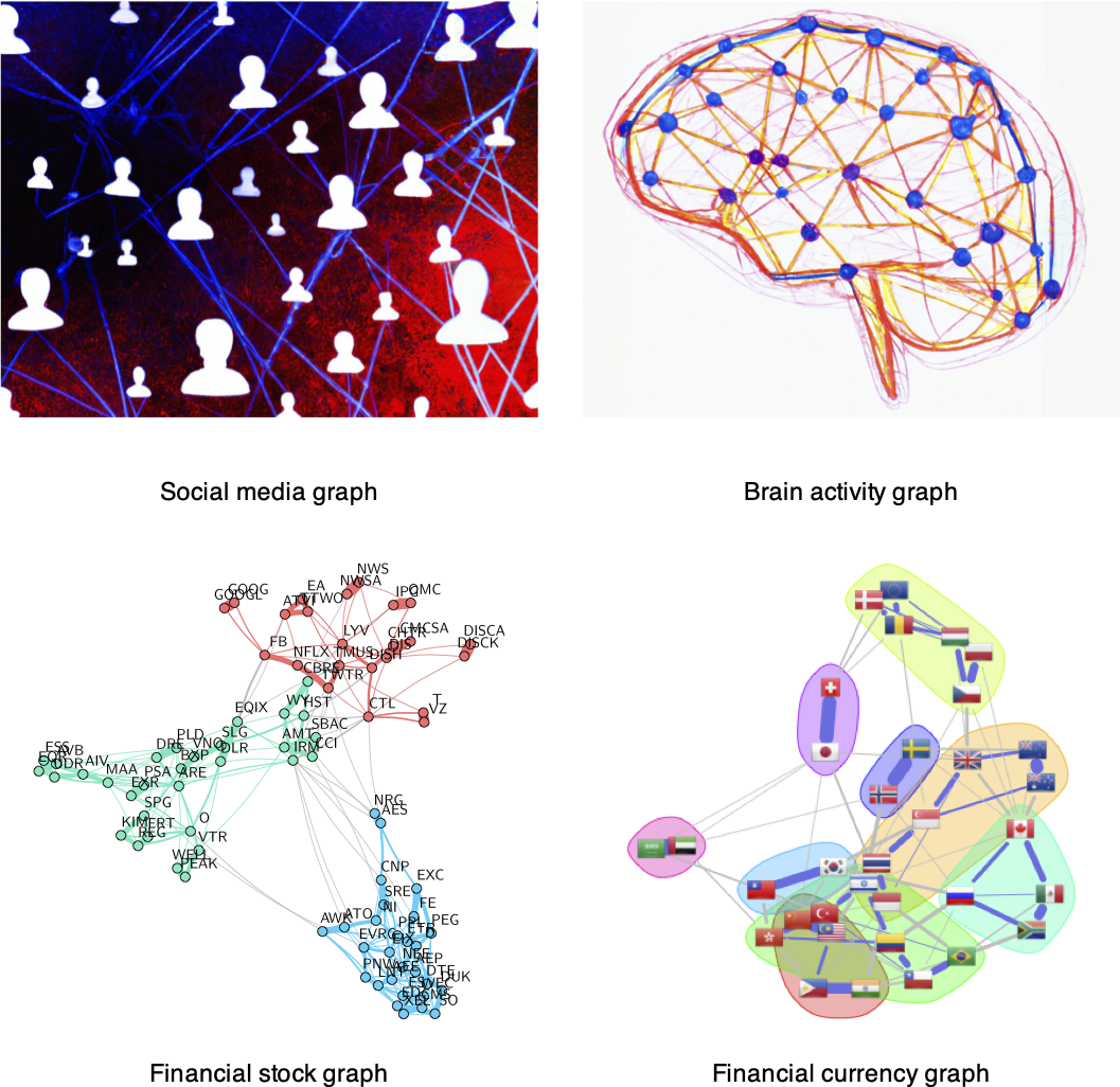
Figure 5.1: Examples of graphs in different applications.
5.1.1 Terminology
The basic elements of a graph (see Figure 5.2) are
- nodes: corresponding to the entities or variables; and
- edges: encoding the relationships between entities or variables.
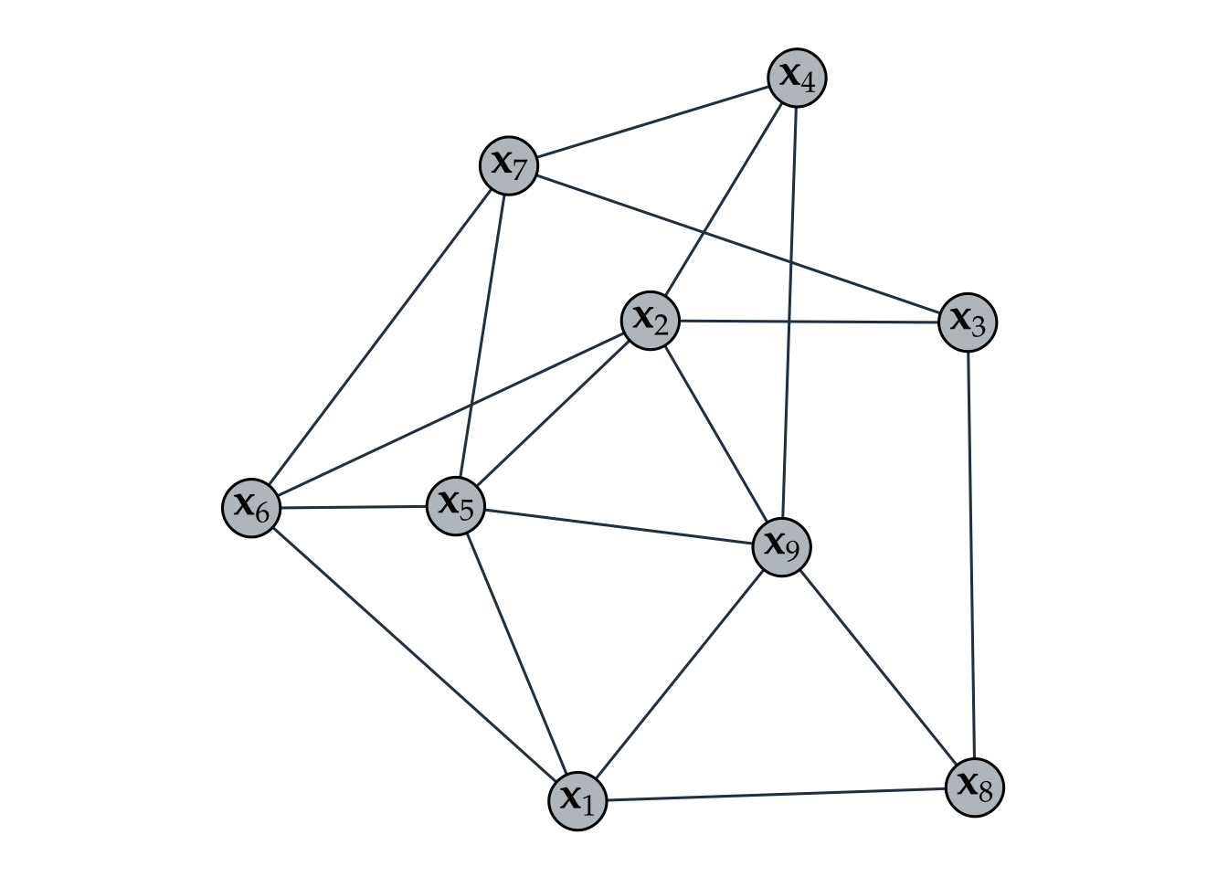
Figure 5.2: Illustration of a graph with nodes and edges.
A graph is a simple mathematical structure described by \(\mathcal{G}=(\mathcal{V},\mathcal{E},\bm{W})\), where the set \(\mathcal{V}=\{1,2,3,\ldots,p\}\) contains the indices of the nodes, the set of pairs \(\mathcal{E}=\{(1,2),{(1,3)},\ldots,{(i,j)},\ldots\}\) contains the edges between any pair of nodes \((i,j)\), and the weight matrix \(\bm{W}\) encodes the strength of the relationships.
5.1.2 Graph Matrices
Several matrices are key in characterizing graphs.
- The adjacency matrix \(\bm{W}\) is the most direct way to fully characterize a graph, where each element \(W_{ij}\) contains the strength of the connectivity, \(w_{ij}\), between node \(i\) and node \(j\): \[ [\bm{W}]_{ij}=\begin{cases} w_{ij} & \textm{if}\;(i,j)\in\mathcal{E},\\ 0 & \textm{if}\;(i,j)\notin\mathcal{E},\\ 0 & \textm{if}\;i=j. \end{cases} \] We tacitly assume \(W_{ij}\ge0\) and \(W_{ii} = 0\) (no self-loops). If \(W_{ij}=W_{ji}\) (symmetric matrix \(\bm{W}\)), then the graph is called undirected.
- The connectivity matrix \(\bm{C}\) is a particular case of the adjacency matrix containing elements that are either 0 or 1: \[ [\bm{C}]_{ij}=\begin{cases} 1 & \textm{if}\;(i,j)\in\mathcal{E},\\ 0 & \textm{if}\;(i,j)\notin\mathcal{E},\\ 0 & \textm{if}\;i=j. \end{cases} \] It describes the connectivity pattern of the adjacency matrix. In fact, for some graphs the adjacency matrix is already binary (with no measure of strength) and coincides with the connectivity matrix.
- The degree matrix \(\bm{D}\) is defined as the diagonal matrix containing the degrees of the nodes \(\bm{d} = (d_1,\dots,d_p)\) along the diagonal, where the degree of a node \(i\), \(d_i\), represents its overall connectivity strength to all the nodes, that is, \(d_i = \sum_{j} W_{ij}\). In other words, \[\bm{D}=\textm{Diag}(\bm{W}\bm{1}).\]
- The Laplacian matrix of a graph is defined as \[\bm{L} = \bm{D} - \bm{W}.\] It is also referred to as the combinatorial Laplacian matrix to distinguish it from other variations in the definition of \(\bm{L}.\)
The Laplacian matrix may appear unusual at first; however, it possesses numerous valuable properties that make it a fundamental matrix in graph analysis. It satisfies the following mathematical properties:
- it is symmetric and positive semidefinite: \(\bm{L}\succeq\bm{0}\);
- it has a zero eigenvalue with corresponding eigenvalue the all-one vector \(\bm{1}\): \(\bm{L}\bm{1} = \bm{0}\);
- the degree vector is found along its diagonal: \(\textm{diag}(\bm{L})=\bm{d}\);
- the number of zero eigenvalues corresponds to the number of connected components of the graph (i.e., clusters);
- it defines a measure for the smoothness or variance of graph signals.
To further elaborate on the smoothness property of the Laplacian matrix, let \(\bm{x}=(x_1,\dots,x_p)\) denote a graph signal (i.e., one observation of the signal on all the nodes of the graph). Ignoring the graph, one way to measure the variance of this signal \(\bm{x}\) is with the quantity \(\sum_{i,j}(x_i - x_j)^2.\) Now, to take into account the graph information in this computation, it makes sense to compute the variance between signals \(x_i\) and \(x_j\) only if these two nodes are connected, for example, by weighting the variance between each pair of nodes with the connectivity strength as \(\sum_{i,j}W_{ij}(x_i - x_j)^2.\) This finally leads us to the connection between the Laplacian matrix and a measure of smoothness or variance of the graph signal as \[\begin{equation} \bm{x}^\T\bm{L}\bm{x} = \frac{1}{2}\sum_{i,j}W_{ij}(x_i - x_j)^2. \tag{5.1} \end{equation}\]
Proof. \[\bm{x}^\T\bm{L}\bm{x} = \bm{x}^\T\bm{D}\bm{x} - \bm{x}^\T\bm{W}\bm{x} = \sum_{i}d_{i}x_i^2 - \sum_{i,j}w_{ij}x_ix_j = \sum_{i,j}w_{ij}x_i^2 - \sum_{i,j}w_{ij}x_ix_j.\]
Example 5.1 (Graph matrices for a toy example) Figure 5.3 shows a simple toy undirected graph \(\mathcal{G}=(\mathcal{V},\mathcal{E},\bm{W})\) with four nodes characterized by \(\mathcal{V}=\{1,2,3,4\}\), \(\mathcal{E}=\{(1,2),(2,1),(1,3),(3,1),(2,3),(3,2),(2,4),(4,2)\}\), and weights \(w_{12}=w_{21}=2\), \(w_{13}=w_{31}=2\), \(w_{23}=w_{32}=3\), \(w_{24}=w_{42}=1\).
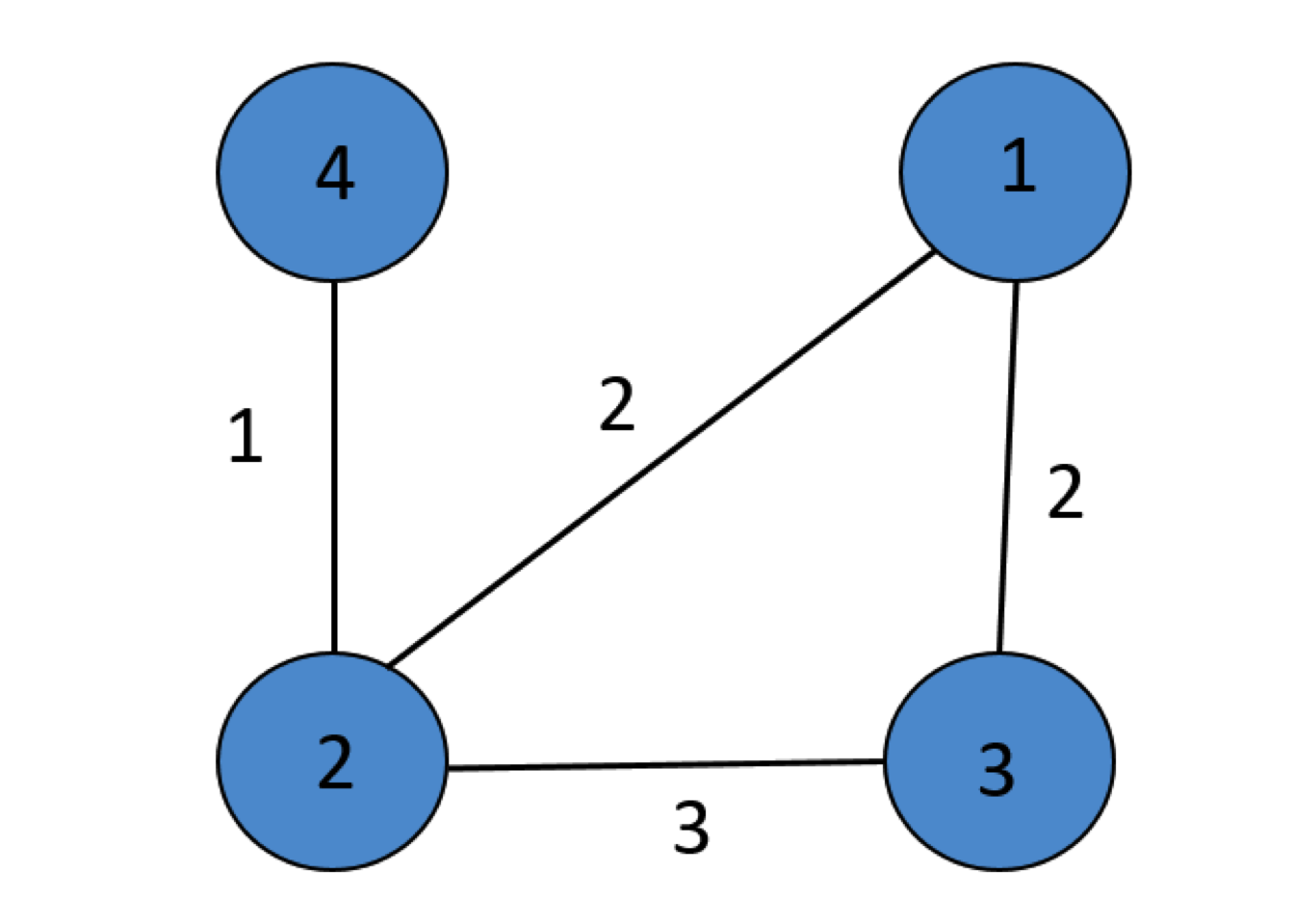
Figure 5.3: Toy graph.
The connectivity, adjacency, and Laplacian graph matrices are \[ \bm{C}=\begin{bmatrix} 0 & 1 & 1 & 0\\ 1 & 0 & 1 & 1\\ 1 & 1 & 0 & 0\\ 0 & 1 & 0 & 0 \end{bmatrix},\quad \bm{W}=\begin{bmatrix} 0 & 2 & 2 & 0\\ 2 & 0 & 3 & 1\\ 2 & 3 & 0 & 0\\ 0 & 1 & 0 & 0 \end{bmatrix},\quad \bm{L}=\begin{bmatrix} 4 & -2 & -2 & 0\\ -2 & 6 & -3 & -1\\ -2 & -3 & 5 & 0\\ 0 & -1 & 0 & 1 \end{bmatrix}. \]