14.1 Introduction
Markowitz’s mean–variance portfolio (Markowitz, 1952) formulates the portfolio design as a trade-off between the expected return \(\w^\T\bmu\) and the risk measured by the variance \(\w^\T\bSigma\w\) (see Chapter 7 for details): \[ \begin{array}{ll} \underset{\w}{\textm{maximize}} & \w^\T\bmu - \frac{\lambda}{2}\w^\T\bSigma\w\\ \textm{subject to} & \w \in \mathcal{W}, \end{array} \] where \((\bmu, \bSigma)\) are the parameters, \(\lambda\) is a hyper-parameter that controls the investor’s risk aversion, and \(\mathcal{W}\) denotes an arbitrary constraint set, such as \(\mathcal{W} = \{\w \mid \bm{1}^\T\w=1, \w\ge\bm{0} \}\).
In practice, the parameters \((\bmu, \bSigma)\) are unknown and have to be estimated using historical data \(\bm{x}_1,\dots,\bm{x}_T\) containing the past \(T\) observations of the assets’ returns. There is a wide span of different estimators, ranging from the simplest sample estimators to the more sophisticated shrinkage heavy-tailed maximum likelihood estimators (see Chapter 3 for a variety of estimation techniques). Regardless of the estimation method employed, there will always be an estimation error that depends on the number of observations. In practice, the amount of available historical data is limited (lack of stationarity does not help either) and the estimates \(\hat{\bmu}\) and \(\hat{\bSigma}\) will be very noisy, particularly \(\hat{\bmu}\) (Best and Grauer, 1991; Chopra and Ziemba, 1993; Michaud, 1989); see Section 3.2 in Chapter 3 for more details.
This is, in fact, the “Achilles’ heel” of portfolio optimization: the estimations \(\hat{\bmu}\) and \(\hat{\bSigma}\) will inevitably contain estimation noise which will lead to erratic portfolio designs. This is why Markowitz’s portfolio has not been fully embraced by practitioners. This was clearly summarized by Michaud in the context of mean–variance formulations (Michaud, 1989):
- Portfolio optimization problems are “estimation-error maximizers.”
- “Optimal” portfolios are financially meaningless (absence of significant investment value).
Figure 14.1 illustrates the sensitivity of the mean–variance portfolio (with \(\lambda=1\)) for six different realizations of the estimation error in the parameters. As can be observed, the behavior is totally erratic because the solutions are too sensitive to the errors in the parameters. In fact, each realization is very different from the others and this is unacceptable from a practical standpoint. One cannot let the portfolio allocation depend on the flap of a butterfly’s wings.
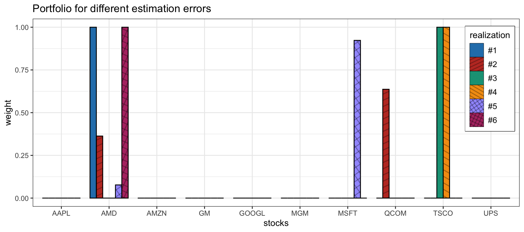
Figure 14.1: Sensitivity of the naive mean–variance portfolio.