3.5 Heavy-Tailed ML Estimators
Gaussian ML estimators are optimal, in the sense of maximizing the likelihood of the observations, whenever data follow the Gaussian distribution. However, if data follow a heavy-tailed distribution – like it is the case with financial data – then we need some further understanding of the potentially detrimental effect. On the one hand, since the ML estimators coincide with the sample estimators in Section 3.2, we know they are unbiased and consistent, which are desirable properties. But, on the other hand, is this sufficient or can we do better?
3.5.1 The Failure of Gaussian ML Estimators
As explored in Section 3.4, Figure 3.6 demonstrates that the effect of heavy tails in the estimation of the covariance matrix is significant, whereas it is almost nonexistent for the estimation of the mean. Figure 3.7 further shows the error as a function of how heavy the tails are (small \(\nu\) represents heavy-tailed distributions whereas large \(\nu\) tends to a Gaussian distribution).
To further understand the detrimental effect of heavy tails, Figure 3.8 illustrates this effect, as well as the effect of outliers in otherwise Gaussian data. In this example, \(T=10\) data points are used for the estimation of the two-dimensional covariance matrix, which satisfies the ratio \(T/N = 5\). It is very clear that, while for Gaussian data the Gaussian ML estimator (or sample covariance matrix) follows the true covariance matrix very closely, once we include a single outlier in the Gaussian data or we use heavy-tailed data, the estimation is disastrous. Still, most practitioners and academics adopt the sample covariance matrix due to its simplicity.
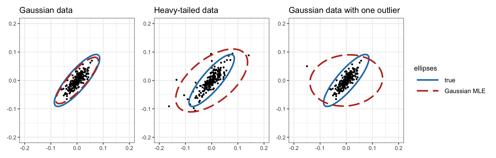
Figure 3.8: Effect of heavy tails and outliers in the Gaussian ML covariance matrix estimator.
3.5.2 Heavy-Tailed ML Estimation
We have empirically observed that the Gaussian MLE for the covariance matrix significantly degrades when the data distribution exhibits heavy tails (see Figures 3.6, 3.7, and 3.8). But this is not unexpected since the sample covariance matrix is optimal only under the Gaussian distribution as derived in Section 3.4. Thus, to derive an improved estimator, we should drop the Gaussian assumption and instead consider a heavy-tailed distribution in the derivation of optimal ML estimators. There are many families of distributions with heavy tails (McNeil et al., 2015) and, for simplicity, we will focus our attention on the Student \(t\) distribution or, simply, \(t\) distribution, which is widely used to model heavy tails via the parameter \(\nu\). It is worth noting that using any other heavy-tailed distribution shows little difference.
The pdf corresponding to the i.i.d. model (3.1), assuming now that the residual term follows a multivariate \(t\) distribution, is \[ f(\bm{x}) = \frac{\Gamma((\nu+N)/2)}{\Gamma(\nu/2)\sqrt{(\nu\pi)^N|\bSigma|}} \left(1 + \frac{1}{\nu}(\bm{x} - \bmu)^\T\bSigma^{-1}(\bm{x} - \bmu)\right)^{-(\nu+N)/2}, \] where \(\Gamma(\cdot)\) is the gamma function,11 \(\bmu\) is the location parameter (which coincides with the mean vector for \(\nu>1\) as in the Gaussian case and is undefined otherwise), \(\bSigma\) denotes the scatter matrix (not to be confused with the covariance matrix, which can now be obtained as \(\frac{\nu}{\nu-2}\bSigma\) if \(\nu>2\) and is undefined otherwise), and \(\nu\) denotes the “degrees of freedom” that controls how heavy or thick the tails are (\(\nu\approx4\) corresponds to significantly heavy tails, whereas \(\nu\rightarrow\infty\) corresponds to the Gaussian distribution). Thus, the parameters of this model are \(\bm{\theta} = (\bmu, \bSigma, \nu)\), which includes the extra scalar parameter \(\nu\) compared to the Gaussian case in (3.4). This parameter can either be fixed to some reasonable value (financial data typically satisfies \(\nu\approx4\) or \(\nu\approx5\)) or can be estimated together with the other parameters.
The MLE can then be formulated, given \(T\) observations \(\bm{x}_1,\dots,\bm{x}_T\), as \[ \begin{array}{ll} \underset{\bmu,\bSigma,\nu}{\textm{minimize}} & \begin{aligned}[t] \textm{log det}(\bSigma) + \frac{\nu+N}{T} \sum_{t=1}^T \textm{log} \left(1 + \frac{1}{\nu}(\bm{x}_t - \bmu)^\T\bSigma^{-1}(\bm{x}_t - \bmu)\right)\\ + 2\;\textm{log}\;\Gamma(\nu/2) + N\textm{log}(\nu) - 2\;\textm{log}\;\Gamma\left(\frac{\nu+N}{2}\right). \end{aligned} \end{array} \]
For simplicity we will fix the parameter \(\nu = 4\), and then only the first two terms in the problem formulation become relevant in the estimation of the remaining parameters \(\bmu\) and \(\bSigma\). Setting the gradient of the objective function with respect to \(\bmu\) and \(\bSigma^{-1}\) to zero leads to \[ \begin{aligned} \frac{1}{T} \sum_{t=1}^T \frac{\nu+N}{\nu + (\bm{x}_t - \bmu)^\T\bSigma^{-1}(\bm{x}_t - \bmu)} (\bm{x}_t - \bmu) &= \bm{0},\\ -\bSigma + \frac{1}{T}\sum_{t=1}^T \frac{\nu+N}{\nu + (\bm{x}_t - \bmu)^\T\bSigma^{-1}(\bm{x}_t - \bmu)} (\bm{x}_t - \bmu)(\bm{x}_t - \bmu)^\T &= \bm{0}, \end{aligned} \] which can be conveniently rewritten as the following fixed-point equations for \(\bmu\) and \(\bSigma\): \[\begin{equation} \begin{aligned} \bmu &= \frac{\frac{1}{T}\sum_{t=1}^T w_t(\bmu,\bSigma) \times \bm{x}_t}{\frac{1}{T}\sum_{t=1}^T w_t(\bmu,\bSigma)},\\ \bSigma &= \frac{1}{T}\sum_{t=1}^T w_t(\bmu,\bSigma) \times (\bm{x}_t - \bmu)(\bm{x}_t - \bmu)^\T, \end{aligned} \tag{3.6} \end{equation}\] where we define the weights \[\begin{equation} w_t(\bmu,\bSigma) = \frac{\nu+N}{\nu + (\bm{x}_t - \bmu)^\T\bSigma^{-1}(\bm{x}_t - \bmu)}. \tag{3.7} \end{equation}\]
It is important to remark that (3.6) are fixed-point equations because the parameters \(\bmu\) and \(\bSigma\) appear on both sides of the equalities, which makes their calculation not trivial. Existence of a solution is guaranteed if \(T > N + 1\) (Kent and Tyler, 1991); conditions for existence and uniqueness with optional shrinkage were derived in Y. Sun et al. (2015).
Nevertheless, these fixed-point equations have a beautiful interpretation: if one assumes the weights \(w_t\) to be known, then the expressions in (3.6) become a weighted version of the Gaussian MLE expressions in (3.5). Interestingly, the weights \(w_t\) have the insightful interpretation that they become smaller as the point \(\bm{x}_t\) is further away from the center \(\bmu\), which means that they automatically down-weight the outliers. Thus, we can expect these estimators to be robust to outliers, unlike the Gaussian ML estimators in (3.5) whose performance can be severely degraded in the presence of outliers. Observe that as \(\nu\rightarrow\infty\), i.e., as the distribution becomes Gaussian, the weights in (3.7) tend to 1 (unweighted case) as expected.
In practice, a simple way to solve the fixed-point equations in (3.6) is via an iterative process whereby the weights are fixed to the most current value and then \(\bmu\) and \(\bSigma\) are updated.12 Specifically, the iterations for \(k=0,1,2,\dots\) are given as follows: \[\begin{equation} \begin{aligned} \bmu^{k+1} &= \frac{\frac{1}{T}\sum_{t=1}^T w_t(\bmu^k,\bSigma^k) \times \bm{x}_t}{\frac{1}{T}\sum_{t=1}^T w_t(\bmu^k,\bSigma^k)},\\ \bSigma^{k+1} &= \frac{1}{T}\sum_{t=1}^T w_t(\bmu^{k+1},\bSigma^k) \times (\bm{x}_t - \bmu^{k+1})(\bm{x}_t - \bmu^{k+1})^\T. \end{aligned} \tag{3.8} \end{equation}\]
The iterative updates in (3.8) can be formally derived from the ML formulation and shown to converge to the optimal solution by means of the MM algorithmic framework. For details on MM, the reader is referred to Y. Sun et al. (2017) and Section B.7 in Appendix B. For the specific derivation of (3.8), together with technical conditions for the convergence of the algorithm, details can be found in Kent et al. (1994) and in Y. Sun et al. (2015) from the MM perspective. For convenience, this MM-based method is summarized in Algorithm 3.1. In addition, the estimation of \(\nu\) is further considered in Liu and Rubin (1995) and acceleration methods for faster convergence are derived in Liu et al. (1998).
Algorithm 3.1: MM-based method to solve the heavy-tailed ML fixed-point equations in (3.6).
Choose initial point \((\bmu^0,\bSigma^0)\);
Set \(k \gets 0\);
repeat
- Iterate the weighted sample mean and sample covariance matrix as \[ \begin{aligned} \bmu^{k+1} &= \frac{\frac{1}{T}\sum_{t=1}^T w_t(\bmu^k,\bSigma^k) \times \bm{x}_t}{\frac{1}{T}\sum_{t=1}^T w_t(\bmu^k,\bSigma^k)},\\ \bSigma^{k+1} &= \frac{1}{T}\sum_{t=1}^T w_t(\bmu^{k+1},\bSigma^k) \times (\bm{x}_t - \bmu^{k+1})(\bm{x}_t - \bmu^{k+1})^\T, \end{aligned} \] where the weights are defined in (3.7);
- \(k \gets k+1\);
until convergence;
Figure 3.9 illustrates the robustness of the heavy-tailed ML estimator, compared with the Gaussian ML estimator, under data with heavy tails and outliers. The difference observed is quite dramatic and should serve as a red flag to practitioners for using the sample covariance matrix when dealing with heavy-tailed data.
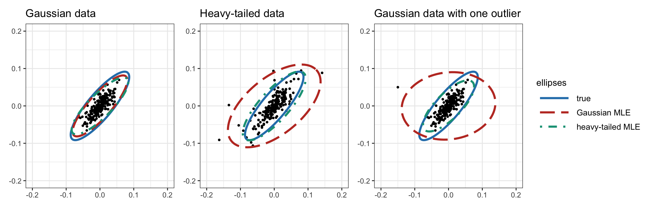
Figure 3.9: Effect of heavy tails and outliers in heavy-tailed ML covariance matrix estimator.
3.5.3 Robust Estimators
What happens if the true distribution that generates the data deviates slightly from the assumed – typically Gaussian – one? Estimators that are not very sensitive to outliers or distribution contamination are generally referred to as robust estimators.
The robustness of estimators can be objectively measured in different ways; notably, with the influence function, which measures the effect when the true distribution slightly deviates from the assumed one, and the breakdown point, which is the minimum fraction of contaminated data points that can render the estimator useless.
As already discussed in Section 3.4, sample estimators or Gaussian ML estimators are not robust against deviations from the Gaussian distribution. It is well known that they are very sensitive to the tails of the distribution (Huber, 1964; Maronna, 1976). In fact, their influence function is unbounded, meaning that an infinitesimal point mass contamination can have an arbitrarily large influence. In addition, a single contaminated point can ruin the sample mean or the sample covariance matrix, that is, the breakdown point is \(1/T\). For reference, the median has a breakdown of around 0.5, that is, one needs more than 50% of the points contaminated to ruin it. On the other hand, as will be further elaborated next, the heavy-tailed ML estimators from Section 3.5.2 can be shown to be robust estimators.
Some classical early references on robust estimation are Huber (1964) for the univariate case and Maronna (1976) for the multivariate case, whereas more modern surveys include Maronna et al. (2006), Huber (2011), Wiesel and Zhang (2014), and Chapter 4 in Zoubir et al. (2018).
\(M\)-Estimators
The term \(M\)-estimators for robust estimation goes back to the 1960s (Huber, 1964). In a nutshell, \(M\)-estimators for the location and scatter parameters, \(\bmu\) and \(\bSigma\), are defined by the following fixed-point equations: \[\begin{equation} \begin{aligned} \frac{1}{T} \sum_{t=1}^T u_1\left(\sqrt{(\bm{x}_t - \bmu)^\T\bSigma^{-1}(\bm{x}_t - \bmu)}\right) (\bm{x}_t - \bmu) &= \bm{0},\\ \frac{1}{T}\sum_{t=1}^T u_2\left((\bm{x}_t - \bmu)^\T\bSigma^{-1}(\bm{x}_t - \bmu)\right) (\bm{x}_t - \bmu)(\bm{x}_t - \bmu)^\T &= \bSigma, \end{aligned} \tag{3.9} \end{equation}\] where \(u_1(\cdot)\) and \(u_2(\cdot)\) are weight functions satisfying some conditions (Maronna, 1976; Maronna et al., 2006).
\(M\)-estimators are a generalization of the maximum likelihood estimators and can be regarded as the weighted sample mean and the weighted sample covariance matrix. In terms of robustness, they have a desirable bounded influence function, although the breakdown point is still relatively low (Maronna, 1976; Maronna et al., 2006). Other estimators, such as the minimum volume ellipsoid and minimum covariance determinant, have higher breakdown points.
The Gaussian ML estimators can be obtained from the \(M\)-estimators in (3.9) with the trivial choice of weight functions \(u_1(s) = u_2(s) = 1\).
A notable common choice to obtain robust estimators is to choose the weight functions based on Huber’s \(\psi\)-function \(\psi(z,k)=\textm{max}(-k,\textm{min}(z,k))\), where \(k\) is a positive constant that caps the argument \(z\) from above and below, as follows (Maronna, 1976): \[ \begin{aligned} u_1(s) &= \psi(z,k)/s,\\ u_2(s) &= \psi(z,k^2)/(\beta s), \end{aligned} \] where \(\beta\) is a properly chosen constant.
Interestingly, the \(M\)-estimators in (3.9) particularize to the heavy-tailed ML estimators derived in (3.7) for the choice \[ u_1(s) = u_2(s^2) = \frac{\nu + N}{\nu + s^2}. \]
Tyler’s Estimator
In 1987, Tyler proposed an estimator for the scatter matrix (which is proportional to the covariance matrix) for heavy-tailed distributions (Tyler, 1987). The idea is very simple and ingenious, as described next. Interestingly, Tyler’s estimator can be shown to be the most robust version of an \(M\)-estimator.
Suppose the random variable \(\bm{x}\) follows a zero-mean elliptical distribution – which means that the distribution depends on \(\bm{x}\) through the term \(\bm{x}^\T\bSigma^{-1}\bm{x}\). If the mean is not zero, then it has to be estimated with some location estimator, as described in Section 3.3, and then subtracted from the observations so that they have zero mean.
The key idea is to normalize the observations \[ \bm{s}_t = \frac{\bm{x}_t}{\|\bm{x}_t\|_2} \] and then use ML based on these normalized points. The surprising fact is that the pdf of the normalized points can be analytically derived – known as angular distribution – as \[ f(\bm{s}) \propto \frac{1}{\sqrt{|\bSigma|}} \left(\bm{s}^\T\bSigma^{-1}\bm{s}\right)^{-N/2}, \] which is independent of the shape of the tails and still contains the parameter \(\bSigma\) which we wish to estimate.
The MLE can then be formulated, given \(T\) observations \(\bm{x}_1,\dots,\bm{x}_T\) and noting that \(\left(\bm{s}_t^\T\bSigma^{-1}\bm{s}_t\right)^{-N/2} \propto \left(\bm{x}_t^\T\bSigma^{-1}\bm{x}_t\right)^{-N/2}\), as \[ \begin{array}{ll} \underset{\bSigma}{\textm{minimize}} & \begin{aligned}[t] \textm{log det}(\bSigma) + \frac{N}{T} \sum_{t=1}^T \textm{log} \left(\bm{x}_t^\T\bSigma^{-1}\bm{x}_t\right). \end{aligned} \end{array} \] Setting the gradient with respect to \(\bSigma^{-1}\) leads to the following fixed-point equation (which has the same form as the one for the heavy-tailed MLE in (3.6)): \[ \bSigma = \frac{1}{T}\sum_{t=1}^T w_t(\bSigma) \times \bm{x}_t \bm{x}_t^\T, \] where the weights are now given by \[\begin{equation} w_t(\bSigma) = \frac{N}{\bm{x}_t^\T\bSigma^{-1}\bm{x}_t}. \tag{3.10} \end{equation}\] Observe that these weights behave similarly to those in (3.7), in the sense of down-weighting the outliers and making the estimator robust. Existence of a solution is guaranteed if \(T > N\) (Tyler, 1987); conditions for existence and uniqueness with optional shrinkage were derived in Y. Chen et al. (2011), Wiesel (2012b), and Y. Sun et al. (2014).
This fixed-point equation can be solved iteratively like in the case of the heavy-tailed MLE in Section 3.5.2, see Tyler (1987) and Y. Sun et al. (2014). However, it is important to realize that Tyler’s method can only estimate the parameter \(\bSigma\) up to a scaling factor, as can be observed from the invariance of the likelihood function with respect to a scaling factor in \(\bSigma\). In fact, this should not be surprising since the normalization of the original points destroys the information of such a scaling factor. In practice, the scaling factor \(\kappa\) can be recovered with some simple heuristic to enforce \[ \textm{diag}(\kappa\times \bSigma) \approx \hat{\bm{\sigma}}^2, \] where \(\hat{\bm{\sigma}}^2\) denotes some robust estimation of the variances of the assets; for example, \[ \kappa = \frac{1}{N}\bm{1}^\T\left(\hat{\bm{\sigma}}^2/\textm{diag}(\bSigma)\right). \]
3.5.4 Numerical Experiments
We now proceed to a final comparison of the presented robust estimators benchmarked against the traditional and popular Gaussian-based estimator. In particular, the following estimators are considered for the mean and covariance matrix:
- Gaussian MLE
- heavy-tailed MLE
- Tyler’s estimator for the covariance matrix (with spatial median for the location).
Figure 3.10 shows the estimation error as a function of the number of observations \(T\) for synthetic heavy-tailed data (\(t\) distribution with \(\nu=4\)). The heavy-tailed MLE is the best, followed closely by the Tyler estimator (with the spatial median estimator for the mean), while the Gaussian MLE is the worst by far.
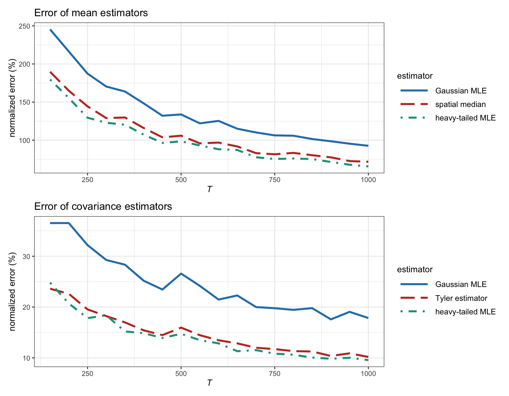
Figure 3.10: Estimation error of different ML estimators vs. number of observations (for \(t\)-distributed heavy-tailed data with \(\nu=4\) and \(N=100\)).
Figure 3.11 examines in more detail the effect of the heavy tails in the estimation error for synthetic data following a \(t\) distribution with degrees of freedom \(\nu\). We can confirm that for Gaussian tails, the Gaussian MLE is similar to the heavy-tailed MLE; however, as the tails become heavier (smaller values of \(\nu\)), the difference becomes quite significant in favor of the robust heavy-tailed MLE.
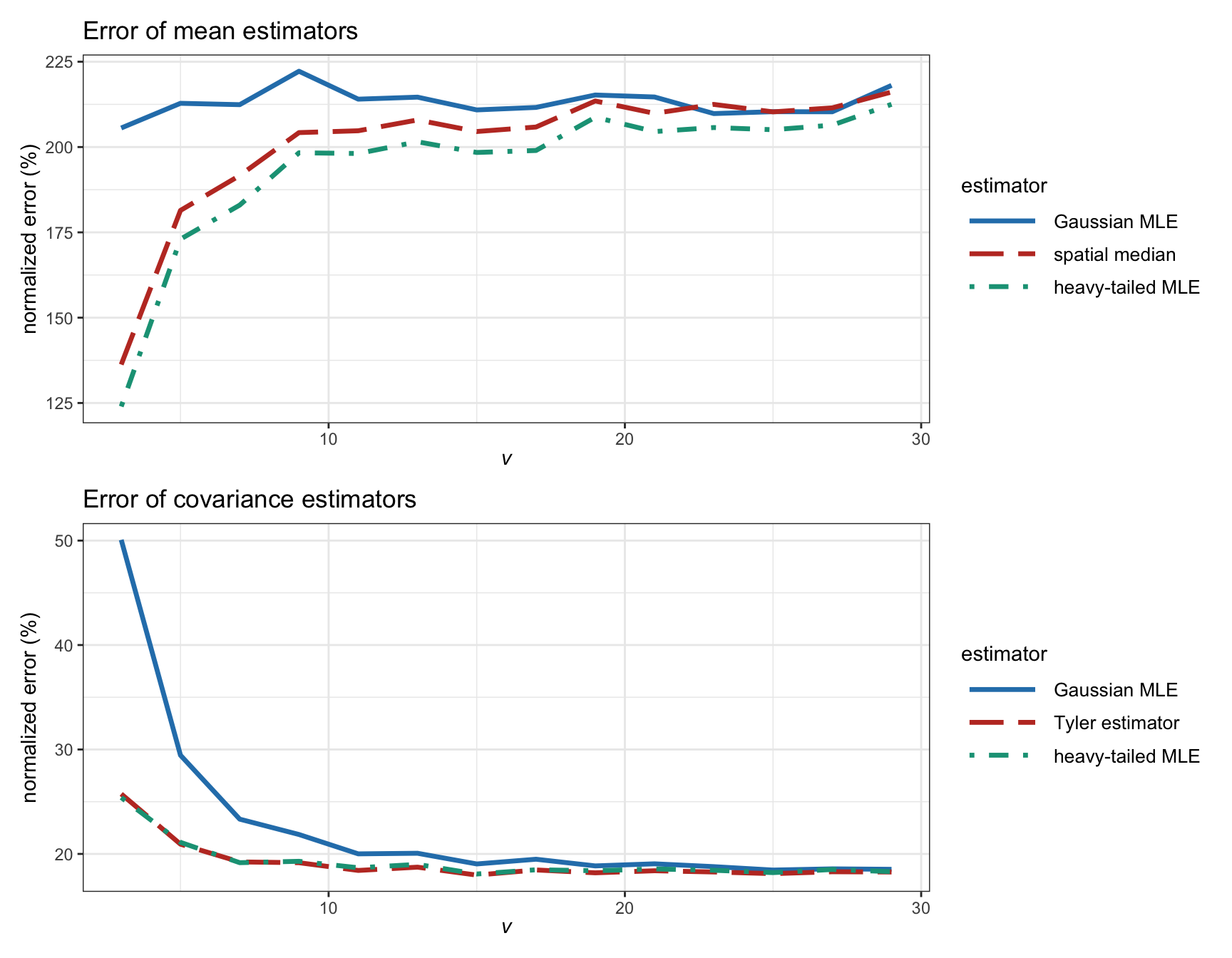
Figure 3.11: Estimation error of different ML estimators vs. degrees of freedom in a \(t\) distribution (with \(T=200\) and \(N=100\)).
The final conclusion could not be more clear: financial data is heavy-tailed and one must necessarily use robust heavy-tailed ML estimators (like the one summarized in Algorithm 3.1). Interestingly, the computational cost of the robust estimators is not much higher than the traditional sample estimators because the algorithm converges in just a few iterations (each iteration has a cost comparable to the sample estimators). Indeed, Figure 3.12 indicates that the algorithm converges in three to five iterations in this particular example with heavy-tailed data (following a \(t\) distribution with \(\nu=4\)) with \(T=200\) observations and \(N=100\) assets.
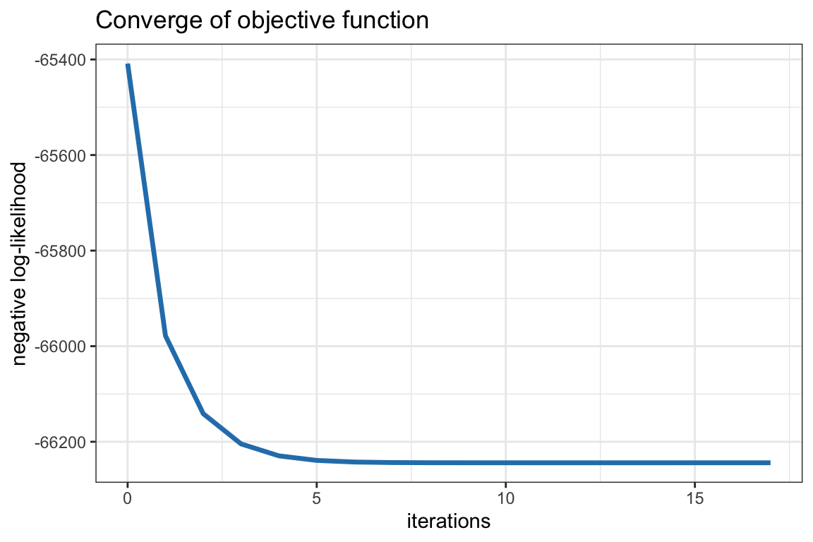
Figure 3.12: Convergence of robust heavy-tailed ML estimators.
Nevertheless, it is important to emphasize that the errors in the estimation of the mean vector \(\bmu\) based on historical data are extremely large (see Figures 3.10 and 3.11), to the point that such estimations may become useless in practice. This is precisely why practitioners typically obtain factors from data providers (at a high premium) and then use them to estimate \(\bmu\) via regression. Alternatively, many portfolio designs that ignore any estimation of \(\bmu\) are quite common, for example the global minimum variance portfolio (see Chapter 6) and the risk parity portfolio (see Chapter 11).
References
The gamma function is defined as \(\Gamma(z) = \int_0^\infty t^{z-1}e^{-t}\,\mathrm{d}t\). For a positive integer \(n\), it corresponds to the factorial function \(\Gamma(n)=(n-1)!\).↩︎
The R package
fitHeavyTailcontains the functionfit_mvt()to solve the fixed-point equations (3.6)-(3.7) iteratively via (3.8) (Palomar et al., 2023). ↩︎