10.3 Downside Risk Portfolios
We now consider portfolio formulations based on downside risk measures.
10.3.1 Formulation
Using the downside risk measure LPM in (10.2) instead of the usual variance \(\w^\T\bSigma\w\) leads to the mean–downside risk formulation: \[\begin{equation} \begin{array}{ll} \underset{\w}{\textm{maximize}} & \w^\T\bmu - \lambda \,\E\left[\left((\tau - \w^\T\bm{r})^+\right)^\alpha\right]\\ \textm{subject to} & \w \in \mathcal{W}. \end{array} \tag{10.7} \end{equation}\] Note that this problem can be similarly formulated by moving either the expected return or risk term to the constraints (see Chapter 7).
In practice, the expectation operator in the LPM has to be approximated by the sample mean over \(T\) observations \(\bm{r}_1, \dots, \bm{r}_T\): \[ \E\left[\left((\tau - \w^\T\bm{r})^+\right)^\alpha\right] \approx \frac{1}{T}\sum_{t=1}^T \left((\tau - \w^\T\bm{r}_t)^+\right)^\alpha. \] Note that this is the same technique used to approximate the variance: \[ \E\left[\left(\w^\T(\bm{r} - \bmu)\right)^2\right] \approx \frac{1}{T}\sum_{t=1}^T \left(\w^\T(\bm{r}_t - \bmu)\right)^2 = \w^\T\hat{\bSigma}\w, \] where \(\hat{\bSigma}\) is the sample covariance matrix (see Chapter 3 for details on estimating the covariance matrix).
Thus, the mean–downside risk formulation is finally written as \[ \begin{array}{ll} \underset{\w}{\textm{maximize}} & \w^\T\bmu - \lambda \frac{1}{T}\sum_{t=1}^T \left((\tau - \w^\T\bm{r}_t)^+\right)^\alpha\\ \textm{subject to} & \w \in \mathcal{W}, \end{array} \] where all the return observations \(\bm{r}_1, \dots, \bm{r}_T\) appear explicitly and cannot be condensed into a convenient matrix (unlike in the case of the variance).
From an optimization perspective, it is convenient to rewrite the formulation without the nondifferentiable operator \((\cdot)^+\) as \[\begin{equation} \begin{array}{ll} \underset{\w,\{s_t\}}{\textm{maximize}} & \w^\T\bmu - \lambda \frac{1}{T}\sum_{t=1}^T s_t^\alpha\\ \textm{subject to} & 0 \le s_t \ge \tau - \w^\T\bm{r}_t, \qquad t=1,\dots,T,\\ & \w \in \mathcal{W}. \end{array} \tag{10.8} \end{equation}\] Interestingly, the class of optimization problems for common choices of \(\alpha\) (assuming that the constraints in \(\mathcal{W}\) are linear) are all convex and can be optimally solved, namely:
- linear program for \(\alpha=1\);
- quadratic program for \(\alpha=2\) (semi-variance portfolio); and
- general convex program for \(\alpha=3\).
10.3.2 Semi-variance Portfolios
As previously mentioned, the variance has a very convenient expression in terms of the covariance matrix \(\bSigma\): \[ \E\left[\left(\w^\T(\bm{r} - \bmu)\right)^2\right] = \w^\T\bSigma\w, \] where \[\bSigma = \E\left[ \left(\bm{r} - \bmu\right) \left(\bm{r} - \bmu\right)^\T \right].\]
The question is whether the semi-variance enjoys a similar property (even as an approximation) so that we can write \[ \E\left[\left((\tau - \w^\T\bm{r})^+\right)^2\right] \approx \w^\T\bm{M}\w \] for some conveniently defined matrix \(\bm{M}\).
In fact, Markowitz himself suggested using the following matrix (Markowitz, 1959), which provides an exact semi-variance: \[ \bm{M}(\w) = \E\left[ (\tau\bm{1} - \bm{r}) (\tau\bm{1} - \bm{r})^\T \times I\{\tau > \w^\T\bm{r}\}\right], \] where \(\bm{1}\) denotes the all-one vector and \(I\{\cdot\}\) the indicator function. However, this matrix is endogenous in the sense that it depends on the portfolio \(\w\) and it is therefore not appropriate for portfolio optimization.
Unfortunately, the semi-variance cannot be written via an exogenous matrix \(\bm{M}\) (independent of \(\w\)). Nevertheless, this has not stopped authors from proposing good heuristic approximations (Estrada, 2008) such as \[ \bm{M} = \E\left[ (\tau\bm{1} - \bm{r})^+ \left((\tau\bm{1} - \bm{r})^+\right)^\T \right]. \] Many other practical approaches have been proposed over the past few decades, cf. Estrada (2008).
Summarizing, the mean–semi-variance formulation can be obtained by setting \(\alpha=2\) in (10.7), but it can also be conveniently approximated (similarly to the mean–variance formulation) as \[ \begin{array}{ll} \underset{\w}{\textm{maximize}} & \w^\T\bmu - \frac{\lambda}{2} \w^\T\bm{M}\w\\ \textm{subject to} & \w \in \mathcal{W}. \end{array} \]
10.3.3 Numerical Experiments
We now compare different versions of downside risk portfolios based on (10.8), namely, for \(\alpha=1\), \(\alpha=2\) (with and without the approximation), and \(\alpha=3\). To focus on the effect of the risk measure, we ignore the expected return term in the optimization (effectively letting \(\lambda\rightarrow\infty\)) and also include the GMVP as a reference benchmark.
Figure 10.5 shows boxplots of the Sharpe ratio and maximum drawdown for 200 realizations of 50 randomly chosen stocks from the S&P 500 during 2015–2020, reoptimizing the portfolios every month with a lookback of one year.
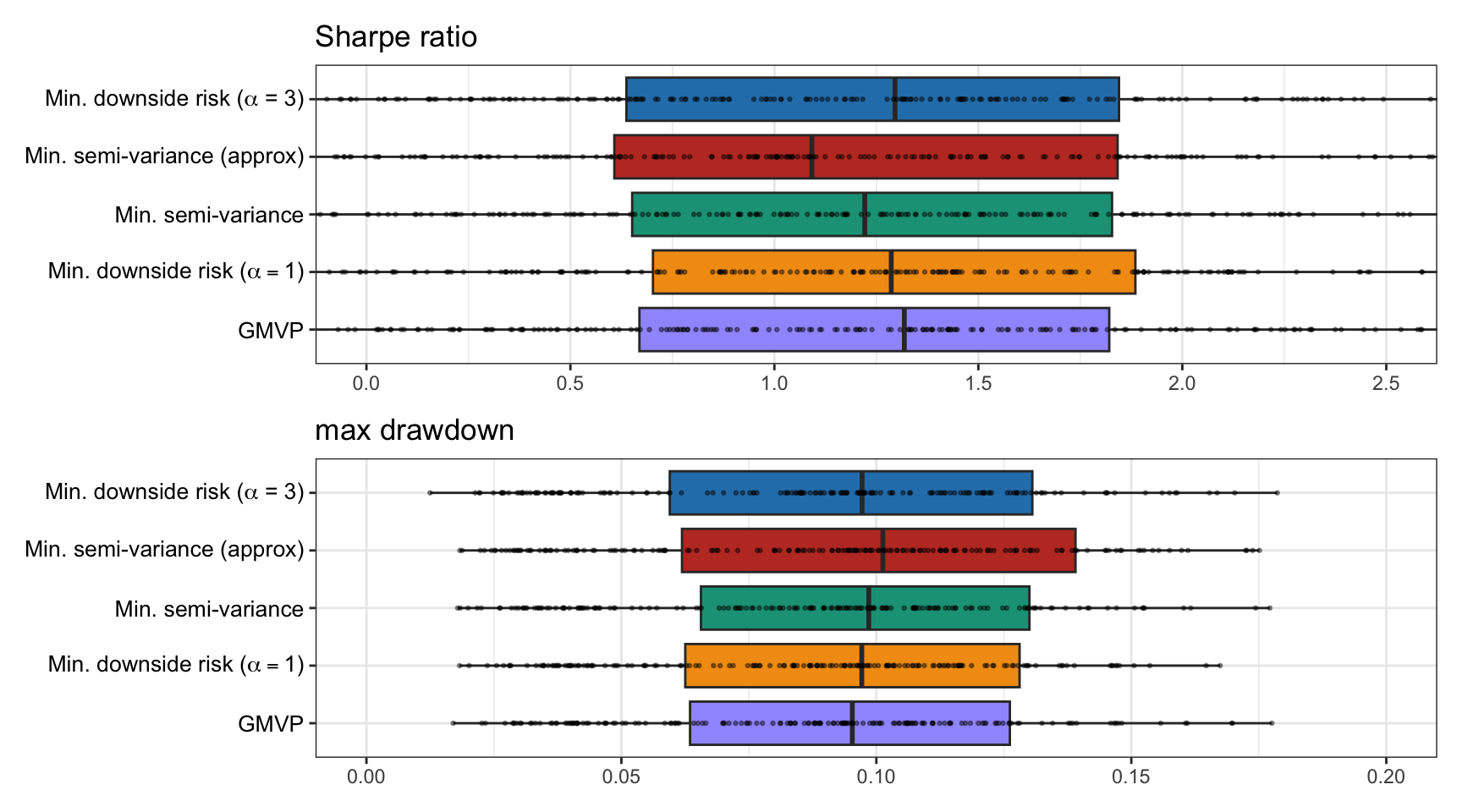
Figure 10.5: Backtest performance of different downside risk portfolios.