B.10 Numerical Comparison
We will now compare the different algorithms with the \(\ell_2\)–\(\ell_1\)-norm minimization example (Zibulevsky and Elad, 2010): \[ \begin{array}{ll} \underset{\bm{x}}{\textm{minimize}} & \frac{1}{2}\|\bm{A}\bm{x} - \bm{b}\|_2^2 + \lambda\|\bm{x}\|_1. \end{array} \] To facilitate comparison, we express the iterates of the various algorithms in a uniform manner, utilizing the soft-thresholding operator \(\mathcal{S}\) as defined in (B.11).
BCD (a.k.a. Gauss–Seidel) iterates: \[ \bm{x}^{k+1} = \mathcal{S}_{\frac{\lambda}{\textm{diag}(\bm{A}^\T\bm{A})}}\left(\bm{x}^k - \frac{\bm{A}^\T\left(\bm{A}\bm{x}^{(k,i)} - \bm{b}\right)}{\textm{diag}\left(\bm{A}^\T\bm{A}\right)}\right), \qquad i=1,\dots,n,\quad k=0,1,2,\dots, \] where \(\bm{x}^{(k,i)} \triangleq \left(x_1^{k+1},\dots,x_{i-1}^{k+1}, x_{i}^{k},\dots,x_{n}^{k}\right).\)
Parallel version of BCD (a.k.a. Jacobi) iterates: \[ \bm{x}^{k+1} = \mathcal{S}_{\frac{\lambda}{\textm{diag}(\bm{A}^\T\bm{A})}}\left(\bm{x}^k - \frac{\bm{A}^\T\left(\bm{A}\bm{x}^{k} - \bm{b}\right)}{\textm{diag}\left(\bm{A}^\T\bm{A}\right)}\right), \qquad i=1,\dots,n,\quad k=0,1,2,\dots \]
MM iterates: \[ \bm{x}^{k+1} = \mathcal{S}_{\frac{\lambda}{\kappa}} \left( \bm{x}^k - \frac{1}{\kappa}\bm{A}^\T\left(\bm{A}\bm{x}^k - \bm{b}\right) \right), \qquad k=0,1,2,\dots \]
Accelerated MM iterates: \[ \left. \begin{aligned} \bm{r}^k &= R(\bm{x}^k) \triangleq \textm{MM}(\bm{x}^k) - \bm{x}^k\\ \bm{v}^k &= R(\textm{MM}(\bm{x}^k)) - R(\bm{x}^k)\\ \alpha^k &= -\textm{max}\left(1, \|\bm{r}^k\|_2/\|\bm{v}^k\|_2\right)\\ \bm{y}^k &= \bm{x}^k - \alpha^k \bm{r}^k\\ \bm{x}^{k+1} &= \textm{MM}(\bm{y}^k) \end{aligned} \quad \right\} \qquad k=0,1,2,\dots \]
SCA iterates: \[ \left. \begin{aligned} \hat{\bm{x}}^{k+1} &= \mathcal{S}_{\frac{\lambda}{\tau + \textm{diag}(\bm{A}^\T\bm{A})}} \left(\bm{x}^k - \frac{\bm{A}^\T\left(\bm{A}\bm{x}^k - \bm{b}\right)}{\tau + \textm{diag}\left(\bm{A}^\T\bm{A}\right)}\right)\\ \bm{x}^{k+1} &= \gamma^k \hat{\bm{x}}^{k+1} + \left(1 - \gamma^k\right) \bm{x}^{k} \end{aligned} \quad \right\} \qquad k=0,1,2,\dots \]
ADMM iterates: \[ \left. \begin{aligned} \bm{x}^{k+1} &= \left(\bm{A}^\T\bm{A} + \rho\bm{I}\right)^{-1}\left(\bm{A}^\T\bm{b} +\rho\left(\bm{z}^k - \bm{u}^k\right)\right)\\ \bm{z}^{k+1} &= \mathcal{S}_{\lambda/\rho} \left(\bm{x}^{k+1} + \bm{u}^k\right)\\ \bm{u}^{k+1} &= \bm{u}^{k} + \left(\bm{x}^{k+1} - \bm{z}^{k+1}\right) \end{aligned} \quad \right\} \qquad k=0,1,2,\dots \]
Observe that BCD updates each element sequentially, whereas all the other methods update all the elements simultaneously (this translates into an unacceptable increase in the computational cost for BCD).
The Jacobi update is the parallel version of BCD, although in principle it is not guaranteed to converge. Interestingly, the Jacobi update looks strikingly similar to the SCA update, except that SCA includes \(\tau\) and the smoothing step, which are precisely the necessary ingredients to guarantee convergence.
A hidden but critical detail in the MM method is the need to compute the largest eigenvalue of \(\bm{A}^\T\bm{A}\) to be able to choose the parameter \(\kappa > \lambda_\textm{max}\left(\bm{A}^\T\bm{A}\right)\), which results in an upfront increase in computation. In addition, such a value of \(\kappa\) is a very conservative upper bound used in the update of all the elements of \(\bm{x}\). In SCA, this common conservative value of \(\kappa\) is replaced by the vector \(\textm{diag}\left(\bm{A}^\T\bm{A}\right)\), which is better tailored to each element of \(\bm{x}\) and results in faster convergence.
Figure B.14 compares the convergence of all these methods in terms of iterations, as well as CPU time, for the resolution of the \(\ell_2\)–\(\ell_1\)-norm minimization problem with \(m = 500\) linear equations and \(n = 100\) variables. Note that each outer iteration of BCD involves a sequential update of each element, which results in an extremely high CPU time and the curve lies outside the range of the plot. Observe that ADMM converges with a much lower accuracy than the other methods.
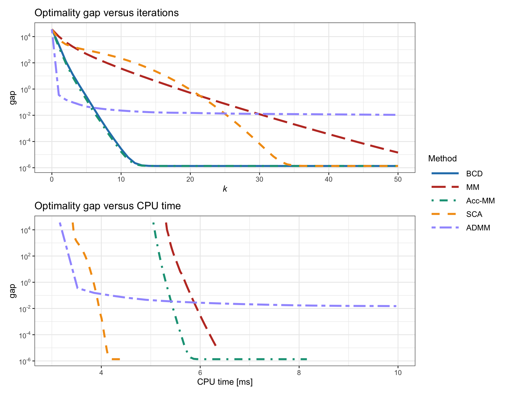
Figure B.14: Comparison of different iterative methods for the \(\ell_2\)–\(\ell_1\)-norm minimization.