15.7 Statistical Arbitrage
Pairs trading focuses on discovering cointegration and tracking the cointegration relationship between pairs of assets. However, the idea can be naturally extended to more than two assets for more flexibility. This is more generally referred to as statistical arbitrage or, for short, StatArb.
Cointegration for more than two assets follows essentially the same idea: construct a linear combination of multiple time series such that the combination is mean reverting. The difference is that the mathematical modeling to capture the multiple cointegration relationships becomes more involved.
15.7.1 Least Squares
Least squares can still be used to determine the cointegration relationship. In the case of \(K>2\) time series, we still need to choose the one to be regressed by the others. Suppose we want to fit \(y_{1t} \approx \mu + \sum_{k=2}^K \gamma_k \, y_{kt}\) based on \(T\) observations. Then, the least squares formulation is \[ \begin{array}{ll} \underset{\mu,\bm{\gamma}}{\textm{minimize}} & \left\Vert \bm{y}_1 - \left(\mu \bm{1} + \bm{Y}_2 \bm{\gamma}\right) \right\Vert_2^2, \end{array} \] where the vector \(\bm{y}_1\) contains the \(T\) observations of the first time series, the matrix \(\bm{Y}_2\) contains the \(T\) observations of the remaining \(K-1\) time series columnwise, and vector \(\bm{\gamma} \in \R^{K-1}\) contains the \(K-1\) hedge ratios. The solution gives the estimates \[ \begin{bmatrix} \begin{array}{ll} \hat{\mu} \\ \hat{\bm{\gamma}} \end{array} \end{bmatrix} = \begin{bmatrix} \begin{array}{ll} \bm{1}^\T\bm{1} & \bm{1}^\T\bm{Y}_2\\ \bm{Y}_2^\T\bm{1} & \bm{Y}_2^\T\bm{Y}_2 \end{array} \end{bmatrix}^{-1} \begin{bmatrix} \begin{array}{ll} \bm{1}^\T\bm{y}_1\\ \bm{Y}_2^\T\bm{y}_1 \end{array} \end{bmatrix}. \] In practice, this estimation process has to be performed on a rolling-window basis to adapt to the slow changes over time.
The normalized portfolio (with leverage 1) is \[\w = \frac{1}{1+\|\bm{\gamma}\|_1}\begin{bmatrix} \;\;\;1\\ -\bm{\gamma} \end{bmatrix},\] with corresponding normalized spread \(z_{t} = \w^\T\bm{y}_{t}\).
It is important to point out that this approach produces a single cointegration relationship, but there may be others that have gone unnoticed. One approach could be to iteratively try to capture more cointegration relationships orthogonal to the previously discovered ones. In addition, this method requires choosing one time series (out of the \(K\) possible ones) to be regressed. In practice, the discovery of multiple cointegration relationships is better achieved by the more sophisticated VECM modeling described next.
15.7.2 VECM
A very common model in econometrics for a multivariate time series (typically denoting the log-prices of \(N\) assets), \(\bm{y}_1,\bm{y}_2,\bm{y}_3,\dots\), is based on taking the first-order difference, \(\Delta \bm{y}_t = \bm{y}_t - \bm{y}_{t-1}\), and then using a vector autoregressive (VAR) model of order \(p\): \[ \Delta \bm{y}_t = \bm{\phi}_0 + \sum_{i=1}^p \bm{\Phi}_i \Delta \bm{y}_{t-i} + \bm{\epsilon}_t, \] where the parameters of the model are \(\bm{\phi}_0 \in \R^N\), \(\bm{\Phi}_1,\dots,\bm{\Phi}_p\in\R^{N\times N}\), and \(\bm{\epsilon}_t\) is the innovation term (see Section 4.3 in Chapter 4 for details). This approach has the feature that due to the differencing it is a stationary model. Unfortunately, this differencing may also destroy some interesting structure in the original data.
The vector error correction model (VECM) (Engle and Granger, 1987) was proposed as a way to apply the VAR model directly on the original sequence without differencing, with the potential danger of lack of stationarity. Employing the VAR model on the original series \(\bm{y}_t\) and rewriting it in terms of \(\Delta \bm{y}_t\) leads to the more refined model \[\begin{equation} \Delta \bm{y}_t = \bm{\phi}_0 + \bm{\Pi}\bm{y}_{t-1} + \sum_{i=1}^{p-1} \tilde{\bm{\Phi}}_i \Delta \bm{y}_{t-i} + \bm{\epsilon}_t, \tag{15.6} \end{equation}\] where the matrix coefficients \(\bm{\Pi} \in \R^{N\times N}\) and \(\tilde{\bm{\Phi}}_1,\dots,\tilde{\bm{\Phi}}_{p-1} \in \R^{N\times N}\) can be related to the \(\bm{\Phi}_i\) used in the previous VAR model. This model includes the term \(\bm{\Pi}\bm{y}_{t-1}\) that could potentially make the model nonstationary because the time series \(\bm{y}_t\) is nonstationary. However, after a careful inspection of (15.6), it is clear that since the left-hand side, \(\Delta \bm{y}_t\), is stationary, so must be the right-hand side, which implies that \(\bm{\Pi}\bm{y}_{t-1}\) must be stationary.
As it turns out, the matrix \(\bm{\Pi}\) is of utmost importance in guaranteeing stationarity of the term \(\bm{\Pi}\bm{y}_{t}\). In general, this matrix will be of low rank, which means that it can be decomposed as the product of two matrices, \[ \bm{\Pi}=\bm{\alpha}\bm{\beta}^\T, \] with \(\bm{\alpha}, \bm{\beta} \in \R^{N\times K}\) having \(K\) columns, where \(K\) is the rank of \(\bm{\Pi}\). This reveals that the nonstationary series \(\bm{y}_t\) (log-prices) becomes stationary after multiplication with \(\bm{\beta}^\T\). In other words, the multivariate time series \(\bm{y}_t\) is cointegrated and each column of matrix \(\bm{\beta}\) produces a different cointegration relationship.
To be more precise, three cases can be identified in terms of the rank of \(\bm{\Pi}\):
- \(K=N\): this means that \(\bm{y}_t\) is already stationary (rarely the case in practice);
- \(K=0\): this means that \(\bm{y}_t\) is not cointegrated (VECM reduces to a VAR model); and
- \(1<K<N\): this is the interesting case that provides \(K\) different cointegration relationships.
Recall that Johansen’s test (Johansen, 1991, 1995) described in Section 15.4 precisely tests the value of the rank of the matrix \(\bm{\Pi}\) arising in the VECM time series modeling.
15.7.3 Optimum Mean-Reverting Portfolio
Least squares and VECM modeling can be conveniently employed to obtain cointegration relationships that produce mean-reverting spreads for pairs trading or statistical arbitrage strategies. In fact, VECM provides us with \(K\) different cointegration relationships contained in the columns of the matrix \(\bm{\beta} \in \R^{N\times K}\). This means that \(K\) different pairs trading strategies could be run in parallel, fully exploiting all these \(K\) directions in the \(N\)-dimensional space.
Alternatively, an optimization-based approach can be taken to design the portfolio that produces the spread. Since the profit in pairs trading is determined by the product of the number of trades and the threshold, the goal is to maximize the zero-crossing rate (which determines the number of trades) as well as the variance of the spread (which determines the threshold). In practice, several proxies can be used to quantify the zero-crossing rate, producing a variety of problem formulations (Cuturi and d’Aspremont, 2013, 2016; d’Aspremont, 2011).
A combined approach of VECM modeling and the optimization-based approach can also be taken. The \(K\)-dimensional subspace defined by the matrix \(\bm{\beta}\) in VECM modeling can be interpreted as defining a cointegration subspace. From this perspective, any portfolio lying within this subspace will provide a mean-reverting spread. Then, rather than using all the \(K\) dimensions to run \(K\) pairs trading strategies in parallel, one could try to further optimize one or more portfolios within that subspace to obtain the best possible spreads (Z. Zhao and Palomar, 2018; Z. Zhao et al., 2019). Overall, this would imply running fewer strategies in parallel but perhaps with stronger mean reversion.
Mathematically, it is convenient to formulate this problem in terms of a portfolio on the \(K\) spreads rather than on the \(N\) original assets as follows.
- From the \(K\) columns of matrix \(\bm{\beta}\), we get \(K\) cointegration relationships: \[\bm{\beta}_k\in\R^N, \qquad k=1,\dots,K.\]
- We can then construct \(K\) portfolios (normalized with leverage 1): \[ \w_k = \frac{1}{\|\bm{\beta}_k\|_1} \bm{\beta}_k, \qquad k=1,\dots,K. \]
- From these portfolios, we can compute the \(K\) spreads from the original time series \(\bm{y}_{t}\in\R^{N}\): \[ z_{kt} = \w_k^\T\bm{y}_{t}, \qquad k=1,\dots,K, \] or, more compactly, \[ \bm{z}_t = \left[\w_1 \dots \w_K \right]^\T \bm{y}_{t} \in \R^{K}. \]
- At this point, we can conveniently optimize a \(K\)-dimensional portfolio \(\w_z \in \R^{K}\) on the spreads \(\bm{z}_t\), from which the overall portfolio to be executed on the underlying assets \(\bm{y}_t\) can be recovered as \[ \w^\textm{overall} = \left[\w_1 \dots \w_K \right] \times \w_z. \]
We can now focus on the optimization of the spread portfolio \(\w_z\) defined on the spreads \(\bm{z}_t\) (Z. Zhao and Palomar, 2018; Z. Zhao et al., 2019). To design the spread portfolio, the goal is to optimize some proxy of the zero-crossing rate while controlling the spread variance. Defining for convenience the lagged covariance matrices of the spreads as \[ \bm{M}_i = \E\left[ \left(\bm{z}_{t}-\E[\bm{z}_{t}]\right) \left(\bm{z}_{t+i}-\E[\bm{z}_{t+i}]\right)^\T \right], \qquad i=0,1,2,\dots \] we can express the variance of the resulting spread as \(\w_z^\T \bm{M}_{0} \w_z\). As for the zero-crossing rate, it is not that straightforward to obtain a convenient expression and several proxies have been proposed in the literature (Cuturi and d’Aspremont, 2013, 2016; Z. Zhao and Palomar, 2018; Z. Zhao et al., 2019):
Predictability statistic: This tries to measure the similarity of a random signal to white noise (small predictability means closer to white noise and vice versa). Mathematically, it is defined as the proportion of the signal variance that is predicted by the autoregressive coefficient in an AR(1) model (Box and Tiao, 1977). Assuming that the spreads follow a vector AR(1) model, \(\bm{z}_{t} = \bm{A}\bm{z}_{t-1} + \epsilon_t\) with the autoregressive matrix coefficient given by \(\bm{A}=\bm{M}_1^\T\bm{M}_0^{-1}\), it follows that the predictability statistic for the final spread \(\w_z^\T\bm{z}_t\) can be written as \[ \textm{pre}(\w_z) = \frac{\w_z^\T \bm{A}\bm{M}_0\bm{A}^\T \w_z}{\w_z^\T \bm{M}_{0} \w_z} = \frac{\w_z^\T \bm{M}_1^\T\bm{M}_0^{-1}\bm{M}_1 \w_z}{\w_z^\T \bm{M}_{0} \w_z}. \]
Portmanteau statistic: This also tries to measure the similarity of a random process to white noise. The portmanteau statistic of order \(p\) is defined as \(\sum_{i=1}^p \rho_i^2\), where \(\rho_i\) is the signal autocorrelation at the \(i\)th lag (Box and Pierce, 1970). Applied to our case, the portmanteau statistic for the final spread \(\w_z^\T\bm{z}_t\) is \[ \textm{por}(\w_z) = \sum_{i=1}^p \left(\frac{\w_z^\T \bm{M}_i \w_z}{\w_z^\T \bm{M}_{0} \w_z}\right)^2. \]
Crossing statistic: This is defined as the number of zero crossings of a centered stationary process and is given by \(\textm{arccos}(\rho_1)/\pi\) (Kedem, 1994; Ylvisaker, 1965). Maximizing the number of zero crossings is then equivalent to minimizing \(\rho_1\). For the final spread \(\w_z^\T\bm{z}_t\), the crossing statistic is given by \[ \textm{cro}(\w_z) = \frac{\w_z^\T \bm{M}_1 \w_z}{\w_z^\T \bm{M}_{0} \w_z}. \] The penalized crossing statistic combines \(\textm{cro}(\w_z)\) with \(\textm{por}(\w_z)\) to minimize the high-order autocorrelations (Cuturi and d’Aspremont, 2013, 2016): \[ \textm{pcro}(\w_z) = \frac{\w_z^\T \bm{M}_1 \w_z}{\w_z^\T \bm{M}_{0} \w_z} + \eta \sum_{i=2}^p \left(\frac{\w_z^\T \bm{M}_i \w_z}{\w_z^\T \bm{M}_{0} \w_z}\right)^2, \] where \(\eta\) is a hyper-parameter that controls the high-order penalization term.
To summarize, we can formulate a mean-reverting portfolio to optimize some zero-crossing proxy, such as \(\textm{pcro}(\w_z)\), while fixing the spread variance: \[\begin{equation} \begin{array}{ll} \underset{\w_z}{\textm{minimize}} & \w_z^\T \bm{M}_1 \w_z + \eta \sum_{i=2}^p \left(\w_z^\T \bm{M}_i \w_z\right)^2\\ \textm{subject to} & \w_z^\T \bm{M}_{0} \w_z \ge \nu,\\ & \w_z \in \mathcal{W}, \end{array} \tag{15.7} \end{equation}\] where \(\nu\), \(\eta\) are hyper-parameters, and \(\mathcal{W}\) denotes some portfolio constraints, such as \(\|\w_z\|_2 = 1\) to avoid numerical issues (Cuturi and d’Aspremont, 2013), a sparsity constraint \(\|\w_z\|_0 = k\) (Cuturi and d’Aspremont, 2016), a budget / market exposure constraint \(\bm{1}^\T \w_z = 1 / 0\) (Z. Zhao and Palomar, 2018), a leverage constraint \(\|\w_z\|_1 = 1\) (Z. Zhao et al., 2019) or, even better in practice, a leverage constraint on the overall portfolio (Z. Zhao et al., 2019): \[ \| \left[\w_1 \dots \w_K \right] \times \w_z \|_1 = 1. \]
15.7.4 Numerical Experiments
Market Data: SPY, IVV, and VOO
To illustrate multiple cointegration relationships via VECM modeling, we consider again three ETFs that track the S&P 500 index, namely, Standard & Poor’s Depository Receipts SPY, iShares IVV, and Vanguard’s VOO. As previously verified in Section 15.4, Johansen’s test indicates two cointegration relationships present, which can be exploited via statistical arbitrage.
Figure 15.27 shows the cumulative returns obtained by executing pairs trading on (i) the first (strongest) spread, (ii) the second (weaker) spread, (iii) the optimized spread according to (15.7), and (iv) both spreads in parallel (allocating half of the budget to each spread). It can be observed that the strongest spread is better than the second spread. The optimized spread does not seem to offer an improvement in this particular case (for a larger dimensionality of the cointegrated subspace it may still offer some benefits). Last, but not least, using both spreads in parallel offers a steadier cumulative return (i.e., better Sharpe ratio) as expected from the diversity gain. Table 15.5 provides the Sharpe ratios of the different approaches for a more quantitative comparison.
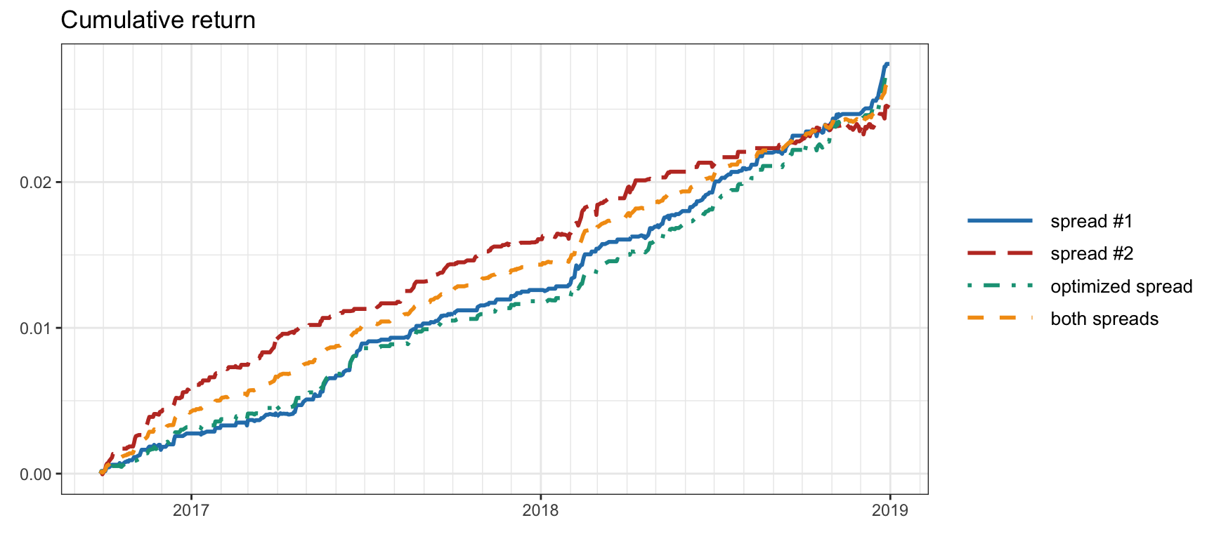
Figure 15.27: Cumulative return for pairs trading on SPY–IVV–VOO: single spreads, both in parallel, and optimized spread.
| Spread | Sharpe ratio |
|---|---|
| Spread #1 | 6.78 |
| Spread #2 | 5.39 |
| Optimized spread | 6.75 |
| Both spreads | 8.37 |