6.4 Heuristic Portfolios
We begin our exploration of portfolios with some heuristic portfolios that may not be formally derived in a mathematically sound manner, but have proven to be widely used by practitioners and can serve as benchmarks.
6.4.1 Buy and Hold Portfolio
One of the simplest investment strategies consists of selecting just one asset and allocating the whole budget to it: \[\begin{equation} \w = \bm{e}_i, \tag{6.9} \end{equation}\] where \(\bm{e}_i\) denotes an all-zero vector with a one at the \(i\)th element. This is called single-asset buy and hold (B&H), which lacks diversification. More generally, the B&H portfolio can be composed of several assets or ETFs, but always with a long horizon so that the portfolio is not adjusted over short horizons.
The belief behind such a strategy is that the asset will increase gradually in value over the investment period. The challenge, naturally, lies in determining which asset to invest in. One can use different methods, like fundamental analysis or technical analysis, to make the choice.
6.4.2 Global Maximum Return Portfolio (GMRP)
The B&H portfolio allocates all the budget to a single asset chosen in a discretionary (e.g., based on expertise, opinion, or technical analysis) or mathematical (e.g., based on fundamental analysis or statistical analysis) manner. Interestingly, if the choice of the top-performing asset is based on the assets’ return forecast \(\bmu\), then it can be formally derived as the optimal portfolio of a poorly chosen cost function, as shown next.
Mathematically, the global maximum return portfolio (GMRP) is formulated as \[\begin{equation} \begin{array}{ll} \underset{\w}{\textm{maximize}} & \w^\T\bmu\\ \textm{subject to} & \bm{1}^\T\w=1, \quad \w\ge\bm{0}. \end{array} \tag{6.10} \end{equation}\]
This problem is convex (in fact, a linear program (LP)) and can be optimally solved with an LP solver. In this case, the solution is trivial: allocate all the budget to the asset with largest return.
As a word of caution, one should not to be fooled by the sound and formal derivation of this portfolio, because it lacks diversification and it will perform poorly. Note that past performance is not a guarantee of future performance, which is related to the extremely noisy estimation of \(\bmu\) in practice (Chopra and Ziemba, 1993).
6.4.3 \(1/N\) Portfolio
One of the most important goals of quantitative portfolio management is to diversify the investment across different assets in a portfolio, typically summarized as “do not put all your eggs in the same basket.” The simplest way to achieve diversification is by allocating the capital equally across all the \(N\) assets: \[\begin{equation} \w = \frac{1}{N}\times\bm{1}, \tag{6.11} \end{equation}\] where \(\bm{1} \in \R^N\) denotes the all-one vector. This strategy is called the equally weighted portfolio (EWP) or \(1/N\) portfolio.
Historically, this strategy or philosophy has been called the “Talmudic rule” (Duchin and Levy, 2009) since the Babylonian Talmud recommended it approximately 1500 years ago: “A man should always place his money, one third in land, a third in merchandise, and keep a third in hand.”
It has gained much interest due to its superior historical performance and the emergence of several equally weighted ETFs (DeMiguel, Garlappi, and Uppal, 2009). For example, Standard & Poor has developed many S&P 500 equally weighted indices. In addition, the \(1/N\) portfolio has been claimed to outperform Markowitz’s mean–variance portfolio considered later in Section 7.1 (DeMiguel, Garlappi, and Uppal, 2009), although other studies disagree with these empirical results (Kritzman et al., 2010).
\(1/N\) Portfolio as an Optimal Robust Portfolio
The \(1/N\) portfolio has been introduced as a common-sense heuristic portfolio for diversification. Interestingly, it was recently shown to correspond to a formally derived optimal portfolio robust to estimation errors in \(\bmu\) (Zhou and Palomar, 2020). The reader is referred to the robust formulation in (6.13) for more details and to Chapter 14 for an extensive treatment of robust portfolios.
6.4.4 Quintile Portfolio
The quintile portfolio is widely used by practitioners. It is similar to the \(1/N\) portfolio in that it allocates equally to the invested assets; however, it only uses the top-performing assets out of the universe of \(N\) assets. In particular, the quintile portfolio selects the top fifth (or 20%) of the assets; however, one could select a different fraction, such as in the quartile portfolio (one fourth or 25% of the assets) or the decile portfolio (one tenth or 10% of the assets). If shorting is desired, then the bottom part of the assets can be short-sold, termed a long–short quintile portfolio.
Suppose the assets have been properly reordered from top to bottom performers (and that \(N\) is divisible by five for the sake of notation). Then, the quintile portfolio can be expressed as \[\begin{equation} \w = \frac{1}{N/5}\begin{bmatrix} \begin{array}{c} 1\\ \vdots\\ 1 \end{array}\\ \begin{array}{c} 0\\ \vdots\\ 0 \end{array} \end{bmatrix} \begin{array}{c} \left.\begin{array}{c} \\ \\ \\ \end{array}\right\} 20\%\\ \left.\begin{array}{c} \\ \\ \\ \end{array}\right\} 80\% \end{array}. \tag{6.12} \end{equation}\]
The crux of the quintile portfolio lies in the ranking of the assets. One can rank the stocks in a multitude of ways, typically based on expensive factors that investment funds purchase at a premium price. It is also called factor investing as it mimics the returns of some common factors (Jurczenko, 2017).
Factor models, such as the capital asset pricing model (CAPM) (Sharpe, 1964) and Fama–French model (Fama and French, 1993), were initially introduced to explain stock returns. Some of the factors used in these models are calculated as the excess returns of assets with attractive characteristics. For example, five well-known factors, namely, value, low size, low volatility, momentum, and quality, may be obtained by ranking the assets according to book-to-price ratio, low market capitalization, low standard deviation, return, and return on equity, respectively (Bender et al., 2013). Empirical studies show that these factors have exhibited excess returns above the market. The quintile portfolio based on the momentum measured by the estimated return in the past few months is one of the most famous ones. A study found that about 77% of 155 mutual funds were actually using such a portfolio over the 1975–1984 period (Grinblatt et al., 1995). Interestingly, some investors might prefer the quintile portfolio based on the opposite of short-term return because they believe in short-term reversals. It has been a widely debated mystery how these simple portfolios defeat the more theoretical-based portfolios.
In the simplest case, if one only has access to publicly available price data, then some common possible ways to rank the assets are according to the following readily available scores:
- expected performance: \[\textm{score}=\bmu;\]
- Sharpe ratios: \[\textm{score}=\dfrac{\bmu}{\sqrt{\textm{diag}\left(\bSigma\right)}};\]
- mean-variance ratios: \[\textm{score}=\dfrac{\bmu}{\textm{diag}\left(\bSigma\right)}.\]
Quintile Portfolio as an Optimal Robust Portfolio
The quintile portfolio has been introduced as a common-sense heuristic portfolio. However, it was recently shown to correspond to a formally derived optimal portfolio robust to estimation errors in \(\bmu\) (Zhou and Palomar, 2020), as briefly described. The reader is referred to Chapter 14 for an extensive treatment of robust portfolios.
Consider a robust formulation of the GMRP in (6.10): \[\begin{equation} \begin{array}{ll} \underset{\w}{\textm{maximize}} & \underset{\bmu\in\mathcal{S}}{\textm{min}}\;\w^\T\bmu\\ \textm{subject to} & \bm{1}^\T\w=1, \quad \w\ge\bm{0}, \end{array} \tag{6.13} \end{equation}\] where the objective function is the worst-case return among the possible return vectors \(\bmu\in\mathcal{S}\), and the uncertainty set \(\mathcal{S}\) is defined as an \(\ell_1\)-norm ball around the estimated value of the returns \(\bm{\hat{\mu}}\), \[\mathcal{S} = \left\{\bm{\hat{\mu}} + \bm{e} \mid \|\bm{e}\|_1 \leq \epsilon\right\},\] with \(\epsilon\) being the size of the uncertainty region.
It turns out that for an appropriate choice of \(\epsilon\), the solution to the robust formulation in (6.13) is precisely the quintile portfolio in (6.12). Furthermore, the \(1/N\) portfolio in (6.11) can also be obtained as the solution to the robust formulation in (6.13) for a sufficiently large value of \(\epsilon\). This theoretical result helps explain the good performance exhibited by the \(1/N\) portfolio and the quintile portfolio in practice, as they are indeed robust portfolios.
6.4.5 Numerical Experiments
We now compare the heuristic GMRP, \(1/N\) portfolio, and quintile portfolio based on different ranking of the stocks, namely, \(\mu\), \(\mu/\sigma\), and \(\mu/\sigma^2\). We consider eight stocks from the S&P 500 during the period 2019–2020, and perform a simple backtest using 70% of the observations as training data while keeping 30% as test data (i.e., out of sample). More realistically, one should do multiple rolling-window backtests (see Chapter 8 for an extensive treatment of backtesting).
Figure 6.12 shows the normalized dollar allocation of the portfolios, where one can observe the difference in diversification. Figure 6.13 shows the out-of-sample backtest results in terms of cumulative P&L and drawdown. While it may initially look from the P&L that the GMRP performs the best, this is deceiving due to the increase in volatility, as can be observed clearly in the drawdown. The \(1/N\) portfolio is the most diversified one and the best in terms of drawdown in this particularly backtest.
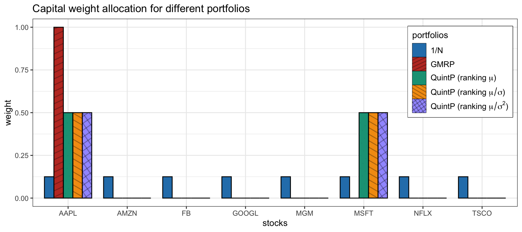
Figure 6.12: Portfolio allocation of some heuristic portfolios.
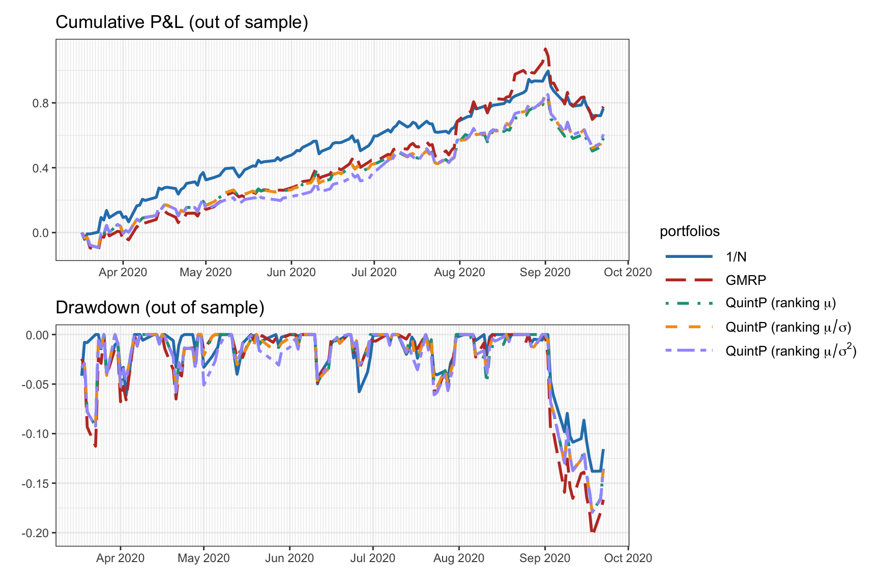
Figure 6.13: Backtest cumulative P&L and drawdown of some heuristic portfolios.