12.4 Numerical Experiments
After looking at several graph-based portfolios and observing their performance over single backtests, we now resort to an empirical evaluation based on multiple randomized backtests. In particular, we take a dataset of the S&P 500 stocks over the period 2015–2020 and generate 200 resamples each with \(N=50\) randomly selected stocks and a random period of two years. Then, for each resample, we perform a walk-forward backtest with a lookback window of one year, reoptimizing the portfolio every month. Note that more exhaustive backtests should be conducted with a wide variety of data before drawing any firm conclusion.
12.4.1 Splitting: Bisection vs. Dendrogram
We start by comparing the two splitting methods considered: direct bisection (after reordering the assets with the dendrogram) and following the natural splits of the dendrogram, as illustrated in Figure 12.12. In principle, one may expect that following the natural dendrogram should be more faithful to the structure in the actual data as opposed to bisection, which somehow breaks the dendrogram. Interestingly, the empirical evaluation in Figure 12.18 seems to suggest otherwise. One possible explanation is that bisection provides more balanced clusters while still using the reordering information provided by the dendrogram.
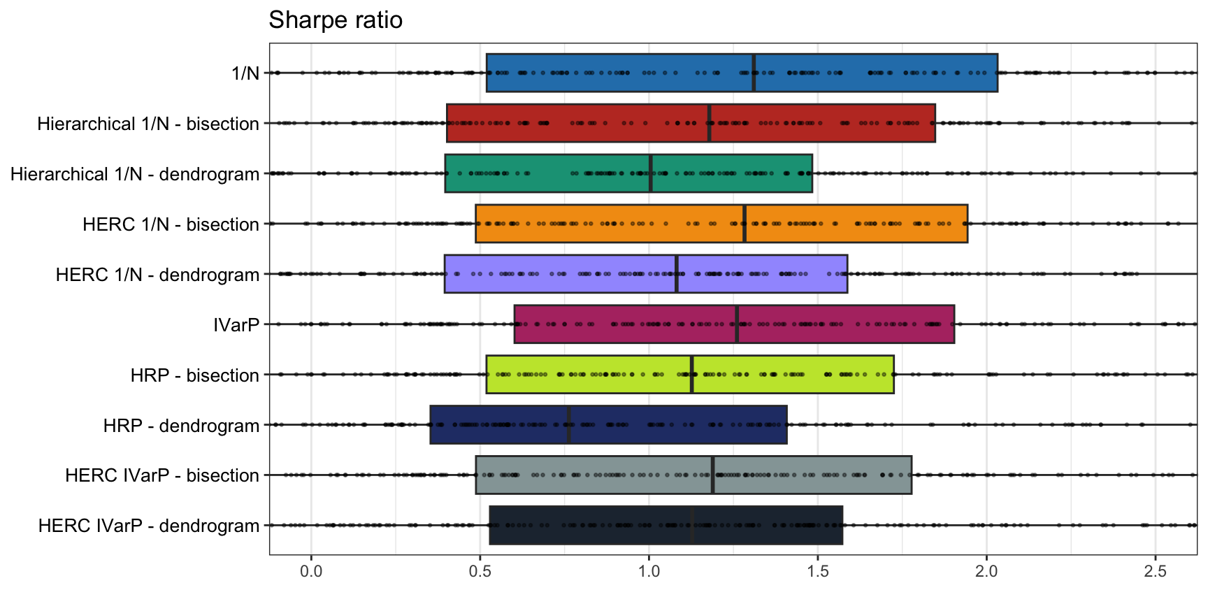
Figure 12.18: Comparison of graph-based portfolios: bisection vs. dendrogram splitting.
12.4.2 Graph Estimation: Simple vs. Sophisticated
Then we evaluate whether the more sophisticated graph estimation methods can bring any benefit to the portfolios. In principle, one may expect a positive answer, but the empirical results in Figure 12.19 show that this is not so clear and further analysis is required.
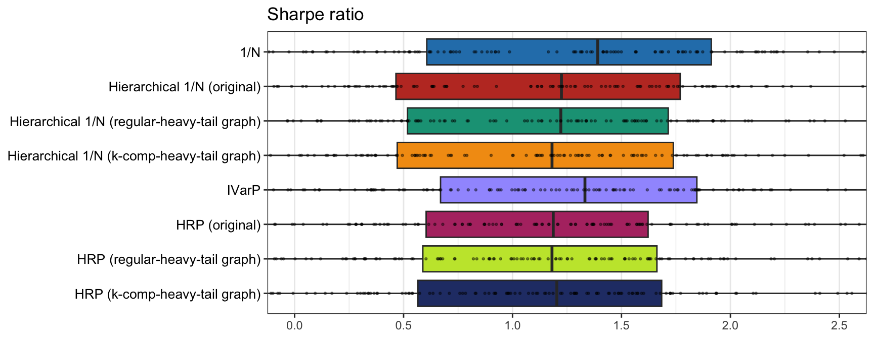
Figure 12.19: Comparison of graph-based portfolios: simple vs. sophisticated graph learning methods.
12.4.3 Final Comparison
Finally, we perform a comparison of the graph-based portfolios (using the simple graph-based distance-of-distance matrix in (12.2)), along with the benchmarks \(1/N\) portfolio and IVarP:
- hierarchical \(1/N\) portfolio
- HERC \(1/N\) portfolio
- HRP portfolio
- HERC IVarP.
The empirical results in Table 12.1 and Figures 12.20–12.21 show that the various methods do not appear significantly different and a more exhaustive comparison is needed before drawing any clear conclusion.
| Portfolio | Sharpe ratio | Annual return | Annual volatility | Sortino ratio | Max drawdown | CVaR (0.95) |
|---|---|---|---|---|---|---|
| 1/\(N\) | 1.01 | 14% | 14% | 1.39 | 11% | 2% |
| Hierarchical 1/\(N\) | 0.81 | 12% | 14% | 1.12 | 11% | 2% |
| HERC 1/\(N\) | 0.99 | 14% | 14% | 1.31 | 11% | 2% |
| IVarP | 1.04 | 13% | 12% | 1.44 | 10% | 2% |
| HRP | 0.91 | 11% | 12% | 1.26 | 10% | 2% |
| HERC IVarP | 0.89 | 12% | 13% | 1.21 | 10% | 2% |
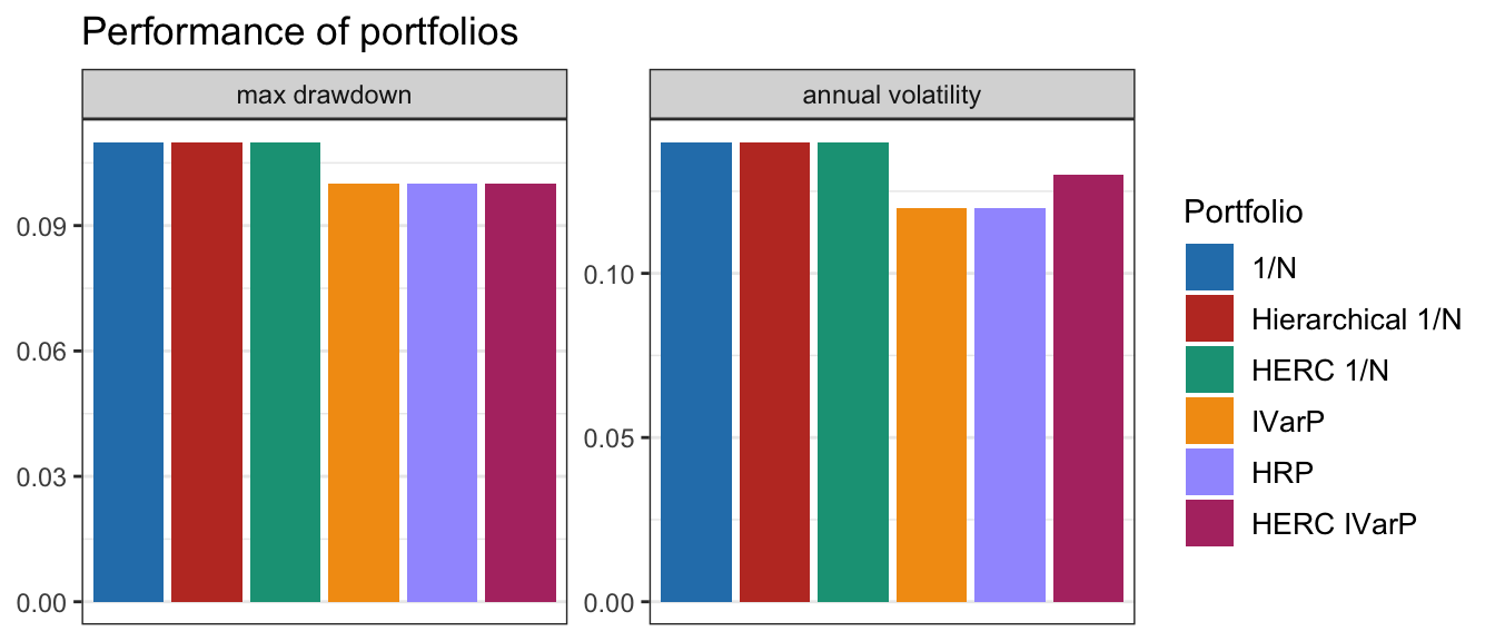
Figure 12.20: Comparison of selected graph-based portfolios: barplots of maximum drawdown and annualized volatility.
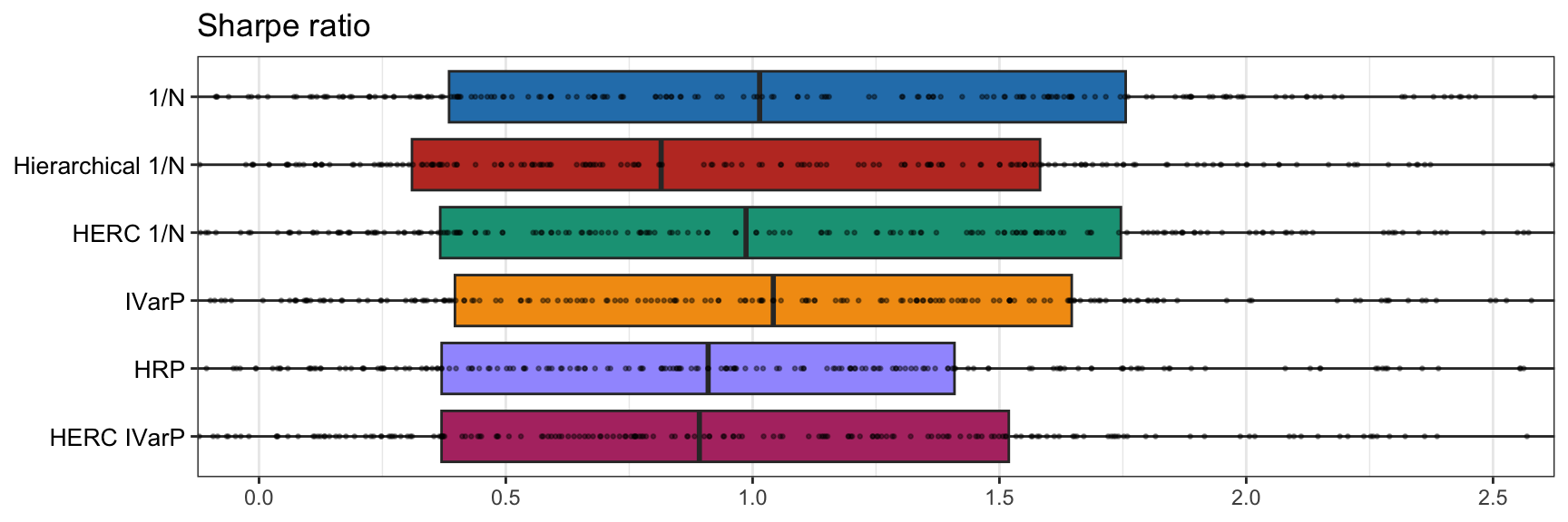
Figure 12.21: Comparison of selected graph-based portfolios: boxplots of Sharpe ratio.