7.4 Universal Algorithm
This chapter has explored a large variety of portfolio formulations with one common theme: they are all based on different combinations of the mean and variance. Even the Kelly criterion-based or utility-based portfolios can be well approximated in terms of the mean and variance. Nevertheless, each of the formulations results in a different type of optimization problem (see the taxonomy of problems in Section A.5). This implies that each formulation requires a different numerical method or solver (see Appendix B for details on algorithms) as listed next:
- scalarized MVP in (7.1): requires a QP solver;
- mean-constrained MVP in (7.3): also needs a QP solver;
- variance-constrained MVP in (7.2): requires a QCQP solver (with a higher computational complexity than a QP solver);
- MSRP in (7.7): this is an FP and can be solved via bisection of SOCPs, via the Dinkelbach sequence of SOCPs, or via the one-shot Schaible transformed QP;
- Kelly portfolio in (7.13): after the approximation in (7.15) this can be solved with a QP solver; and
- utility-based portfolios as in (7.19): also with a QP solver after some mean–variance approximation like in (7.20) or (7.21).
Interestingly, since all such different formulations can be expressed as trade-offs of the mean and variance, the portfolios will naturally lie on the efficient frontier. This means that rather than dealing with each of the formulations separately, an alternative is to solve the basic mean–variance formulation with a properly chosen value of the hyper-parameter \(\lambda\): \[\begin{equation} \begin{array}{ll} \underset{\w}{\textm{maximize}} & \w^\T\bmu - \dfrac{\lambda}{2}\w^\T\bSigma\w\\ \textm{subject to} & \w \in \mathcal{W}, \end{array} \tag{7.23} \end{equation}\] where \(\mathcal{W}\) denotes a general set of constraints for the portfolio (assumed for convenience to contain only linear and quadratic terms, which includes \(\ell_1\)-norms, \(\ell_\infty\)-norms, and \(\ell_2\)-norms). The challenge naturally lies in determining the appropriate value of the hyper-parameter \(\lambda\) (Xiu et al., 2023).
Thus, a general framework can be formulated that embraces all such mean–variance problems as \[\begin{equation} \begin{array}{ll} \underset{\w}{\textm{minimize}} & \begin{array}{l}f\left(\w^\T\bmu, \w^\T\bSigma\w\right)\end{array}\\ \textm{subject to} & \begin{array}[t]{ll} g\left(\w^\T\bmu, \w^\T\bSigma\w\right) \leq 0,\\ \w\in\mathcal{W}, \end{array} \end{array} \tag{7.24} \end{equation}\] where \(f(x,y)\) and \(g(x,y)\) are two functions that consider a trade-off between the two arguments \(x\) and \(y\), which represent the mean and the variance of the portfolio. Table 7.3 shows how \(f(x,y)\) and \(g(x,y)\) particularize to the many mean–variance formulations considered in this chapter.
| Portfolio | \(f(x,y)\) | \(g(x,y)\) |
|---|---|---|
| MVP | \(-x + \frac{\lambda}{2} y\) | — |
| Mean–volatility portfolio | \(-x + \kappa\sqrt{y}\) | — |
| Mean-constrained MVP | \(y\) | \(\beta - x\) |
| Variance-constrained MVP | \(-x\) | \(y - \alpha\) |
| MSRP | \(-\dfrac{x - r_\textm{f}}{\sqrt{y}}\) | — |
| Kelly portfolio | \(-x + \frac{1}{2} y\) | — |
| Kelly portfolio | \(-\textm{log}(1+x) + \frac{1}{2}\dfrac{y}{(1+x)^2}\) | — |
| Kelly portfolio | \(-x + \frac{1}{2}x^2 + \frac{1}{2}\dfrac{y}{1+2x}\) | — |
| Kelly portfolio | \(\begin{aligned}&-\left(1-\frac{1}{\kappa^2}\right)\textm{log}(1+x)\\ &\qquad -\frac{1}{2\kappa^2}\textm{log}\left((1+x)^2 - \kappa^2 y\right)\end{aligned}\) | — |
| Expected utility portfolio | \(-U(0) - U'(0)x - \frac{1}{2}U''(0)(y + x^2)\) | — |
| Expected utility portfolio | \(-U(x) - \frac{1}{2}U''(x)y\) | — |
| Expected utility portfolio | \(-\left(1-\dfrac{1}{\kappa^2}\right)U(x) - \dfrac{U(x + \kappa\sqrt{y}) + U(x - \kappa\sqrt{y})}{2\kappa^2}\) | — |
Notably, it is possible to develop a universal algorithm for mean–variance formulations as in (7.24) (Xiu et al., 2023) with a computational cost orders of magnitude below off-the-shelf general-purpose QP, QCQP, or SOCP solvers. This unified formulation and algorithm provides several practical advantages:
Computational efficiency: It is considerably more efficient to solve a QP than some other more complicated class of problems such as QCQP or SOCP (see Section B.1 for details).
Code reusability: One can devote time and energy to implementing the proper solver function call for problem (7.23), with the advantage that the same code can then be reused for many different formulations as long as they are based on the mean and variance (simply using a different choice of \(\lambda\)).
Code specialization: Rather than using a general-purpose QP solver, an advanced user can develop a tailored numerical algorithm that takes advantage of the particularities of the specific portfolio formulation at hand (this can include the natural sparsity of the long-only portfolio via the active set method or any other numerical trick).
The derivation of the universal algorithm to solve (7.24) is based on the successive convex approximation (SCA) method (Scutari et al., 2014); see Section B.8 in Appendix B for details. In particular, we will successively approximate the problem by a QP, hence the method is called sequential QP (SQP). For the sake of exposition, we will only consider the formulation (7.24) without the constraint function \(g(x,y)\), that is, \[\begin{equation} \begin{array}{ll} \underset{\w}{\textm{minimize}} & f\left(\w^\T\bmu, \w^\T\bSigma\w\right)\\ \textm{subject to} & \w\in\mathcal{W}. \end{array} \tag{7.25} \end{equation}\] For the more general case (7.24), the reader is referred to Xiu et al. (2023).
The idea of SCA (or SQP in this case) is to solve (7.25) by instead solving a sequence of simpler surrogate problems: \[\begin{equation} \begin{array}{ll} \underset{\w}{\textm{minimize}} & \tilde{f}\left(\w;\w^k\right) + \frac{\tau^k}{2} \|\w - \w^k\|_2^2\\ \textm{subject to} & \w\in\mathcal{W}, \end{array} \tag{7.26} \end{equation}\] where \(k\) denotes the iteration index, the surrogate function \(\tilde{f}\left(\w;\w^k\right)\) is a quadratic approximation of \(f\) around the previous point \(\w^k\), and the last term is a quadratic proximal term added to make sure the objective function is strongly convex for convergence reasons (Scutari et al., 2014), which we will take as \(\tau^k=0\). Solving (7.26) sequentially will produce the iterates \(\w^0,\w^1,\w^2,\dots\) until some convergence criterion is satisfied.
The surrogate quadratic function \(\tilde{f}\) can be easily obtained by linearizing the original function \(f\) in terms of \(x=\w^\T\bmu\) and \(y=\w^\T\bSigma\w\), leading to (ignoring the irrelevant constant terms): \[\begin{equation} \tilde{f}\left(\w;\w^k\right) = -\alpha^k \w^\T\bmu + \dfrac{\beta^k}{2} \w^\T\bSigma\w, \tag{7.27} \end{equation}\] where \[\begin{equation} \begin{aligned} \alpha^k &= -\frac{\partial f}{\partial x}\left(x^k=\big(\w^k\big)^\T\bmu, y^k=\big(\w^k\big)^\T\bSigma\w^k\right),\\ \beta^k &= 2\frac{\partial f}{\partial y}\left(x^k=\big(\w^k\big)^\T\bmu, y^k=\big(\w^k\big)^\T\bSigma\w^k\right). \end{aligned} \tag{7.28} \end{equation}\] Table 7.4 shows the expressions of \(\alpha^k\) and \(\beta^k\) for some of the portfolio formulations.
| Portfolio | \(f(x,y)\) | \(\dfrac{\partial f}{\partial x}\) | \(\dfrac{\partial f}{\partial y}\) | \(\alpha^k\) | \(\beta^k\) |
|---|---|---|---|---|---|
| MVP | \(-x + \frac{\lambda}{2} y\) | \(-1\) | \(\lambda/2\) | \(1\) | \(\lambda\) |
| Mean–volatility portfolio | \(-x + \kappa\sqrt{y}\) | \(-1\) | \(\dfrac{\kappa}{2\sqrt{y}}\) | \(1\) | \(\dfrac{\kappa}{\sqrt{(\w^k)^\T\bSigma\w^k}}\) |
| MSRP | \(-\dfrac{x - r_\textm{f}}{\sqrt{y}}\) | \(-\dfrac{1}{\sqrt{y}}\) | \(\dfrac{x - r_\textm{f}}{2y^{3/2}}\) | \(\dfrac{1}{\sqrt{(\w^k)^\T\bSigma\w^k}}\) | \(\dfrac{(\w^k)^\T\bmu - r_\textm{f}}{\left((\w^k)^\T\bSigma\w^k\right)^{3/2}}\) |
| Kelly portfolio | \(-x + \frac{1}{2} y\) | \(-1\) | \(1/2\) | \(1\) | \(1\) |
If we now plug (7.27) into (7.26), after rearranging terms we get \[ \begin{array}{ll} \underset{\w}{\textm{minimize}} & -\w^\T\left(\alpha^k\bmu + \tau^k\w^k\right) + \dfrac{\beta^k}{2} \w^\T\left(\bSigma + \frac{\tau^k}{\beta^k}\bm{I}\right)\w\\ \textm{subject to} & \w\in\mathcal{W}, \end{array} \] which is clearly in the form of the basic mean–variance formulation in (7.23).
Summarizing, we have essentially accomplished our original goal of solving any mean–variance formulation in the form of (7.25) (or, more generally, (7.24)) by solving a sequence of problems like (7.23): \[\begin{equation} \begin{array}{ll} \underset{\w}{\textm{maximize}} & \w^\T\bmu^k - \dfrac{\lambda^k}{2}\w^\T\bSigma^k\w\\ \textm{subject to} & \w \in \mathcal{W}, \end{array} \tag{7.29} \end{equation}\] with \[\begin{equation} \begin{aligned} \bmu^k &= \bmu + \frac{\tau^k}{\alpha^k}\w^k,\\ \bSigma^k &= \bSigma + \frac{\tau^k}{\beta^k}\bm{I},\\ \lambda^k &= \frac{\beta^k}{\alpha^k}. \end{aligned} \tag{7.30} \end{equation}\]
Algorithm 7.3 summarizes this SQP procedure for mean–variance formulations.
Algorithm 7.3: Universal SQP-MVP method to solve (7.25).
Choose initial point \(\w^0 \in \mathcal{W}\), sequences \(\{\tau^k\}\) and \(\{\gamma^k\}\);
Set \(k \gets 0\);
repeat
- Compute \(\alpha^k\) and \(\beta^k\) as in (7.28);
- Compute \(\bmu^k\), \(\bSigma^k\), and \(\lambda^k\) as in (7.30);
- Solve the QP in (7.29) and keep solution as \(\w^{k+1/2}\);
- Set \(\w^{k+1} = \w^k + \gamma_t \left(\w^{k+1/2} - \w^k\right)\);
- \(k \gets k+1\);
until convergence;
Example 7.4 (MSRP) Consider the MSRP formulation \[ \begin{array}{ll} \underset{\w}{\textm{maximize}} & \dfrac{\w^\T\bmu - r_\textm{f}}{\sqrt{\w^\T\bSigma\w}}\\ \textm{subject to} & \begin{array}{l} \bm{1}^\T\w=1, \quad \w\ge\bm{0}.\end{array} \end{array} \] This problem is an FP and can be solved in different ways as covered in Section 7.2. Alternatively, it can be solved via a sequence of simple QPs with Algorithm 7.3 (using \(\tau^k=0\) and \(\gamma^k=1\)) as follows. From Table 7.4, we read the expressions for \(\alpha^k\) and \(\beta^k\), leading to the surrogate mean–variance problem \[ \begin{array}{ll} \underset{\w}{\textm{maximize}} & \w^\T\bmu - \dfrac{\lambda^k}{2}\w^\T\bSigma\w\\ \textm{subject to} & \bm{1}^\T\w=1, \quad \w\ge\bm{0}, \end{array} \] where \(\lambda^k = \beta^k/\alpha^k = \dfrac{(\w^k)^\T\bmu - r_\textm{f}}{(\w^k)^\T\bSigma\w^k}\). Figure 7.7 shows the convergence of this numerical method compared with the solution via the Schaible transform (see Section 7.2), from which we can see that it converges in one to two iterations.
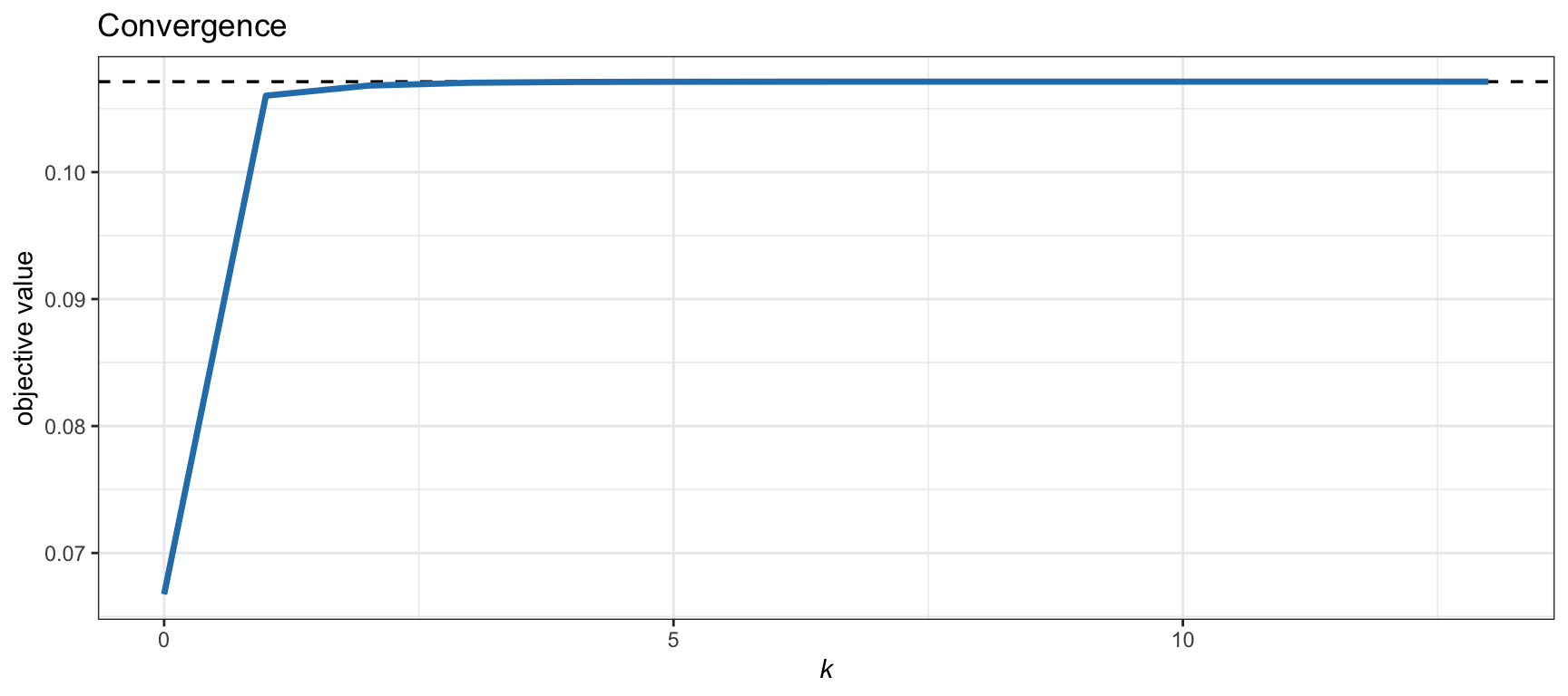
Figure 7.7: Convergence of the SQP-MVP algorithm for the MSRP formulation.
Example 7.5 (Mean--volatility portfolio) Consider the mean–volatility formulation \[ \begin{array}{ll} \underset{\w}{\textm{maximize}} & \w^\T\bmu - \kappa\sqrt{\w^\T\bSigma\w}\\ \textm{subject to} & \bm{1}^\T\w=1, \quad \w\ge\bm{0}, \end{array} \] where \(\kappa\) is a given positive number to control the risk aversion. This problem is a convex SOCP and can be solved with an SOCP solver. Alternatively, it can be solved via a sequence of simple QPs with Algorithm 7.3 (using \(\tau^k=0\) and \(\gamma^k=1\)) as follows. From Table 7.4, we obtain \(\alpha^k = 1\) and \(\beta^k = \kappa/\sqrt{(\w^k)^\T\bSigma\w^k}\), which leads to the surrogate mean–variance problem \[ \begin{array}{ll} \underset{\w}{\textm{maximize}} & \w^\T\bmu - \dfrac{\lambda^k}{2}\w^\T\bSigma\w\\ \textm{subject to} & \bm{1}^\T\w=1, \quad \w\ge\bm{0}, \end{array} \] where \(\lambda^k = \beta^k/\alpha^k = \kappa/\sqrt{(\w^k)^\T\bSigma\w^k}\). Figure 7.8 shows the convergence of this numerical method compared with the solution via an SOCP solver; basically it converges in one iteration.
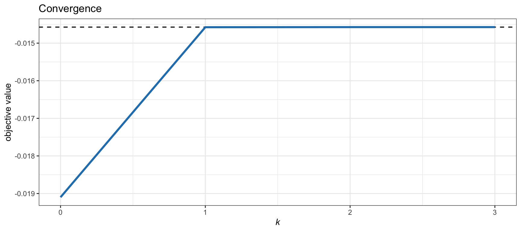
Figure 7.8: Convergence of the SQP-MVP algorithm for the mean–volatility formulation.