3.4 Gaussian ML Estimators
3.4.1 Preliminaries on ML Estimation
Maximum likelihood (ML) estimation is an important technique in estimation theory (T. W. Anderson, 2003; Kay, 1993; Scharf, 1991). The idea is very simple. Suppose the probability of a random variable \(\bm{x}\) can be “measured” by the probability distribution function (pdf) \(f\).10 Then the probability of a series of \(T\) independent given observations \(\bm{x}_1,\dots,\bm{x}_T\) can be measured by the product \(f(\bm{x}_1) \times \cdots \times f(\bm{x}_T)\). Suppose now that we have to guess which of two possible distributions, \(f_1\) and \(f_2\), is more likely to have produced these observations. It seems reasonable to choose as most likely the one that gives the largest probability of observing these observations. Now, suppose we have a family of possible distributions parameterized by the parameter vector \(\bm{\theta}\): \(f_{\bm{\theta}}\), which is called likelihood function when viewed as a function of \(\bm{\theta}\) for the given observations. Again, it seems reasonable to choose as the most likely \(\bm{\theta}\) the one that gives the largest probability of observing these observations. This is precisely the essence of ML estimation and can be written as the following optimization problem: \[ \begin{array}{ll} \underset{\bm{\theta}}{\textm{maximize}} & f_{\bm{\theta}}(\bm{x}_1) \times \cdots \times f_{\bm{\theta}}(\bm{x}_T), \end{array} \] where \(\bm{x}_1,\dots,\bm{x}_T\) denote the \(T\) given observations. For mathematical convenience, ML estimation is equivalently formulated as the maximization of the log-likelihood function: \[ \begin{array}{ll} \underset{\bm{\theta}}{\textm{maximize}} & \begin{aligned}[t] \sum_{t=1}^T \textm{log}\;f_{\bm{\theta}}(\bm{x}_t) \end{aligned}. \end{array} \]
The ML estimator (MLE) enjoys many desirable theoretical properties that make it an asymptotically optimal estimator (asymptotic in the number of observations \(T\)). More specifically, the MLE is asymptotically unbiased and it asymptotically attains the Cramér–Rao bound (which gives the lowest possible variance attainable by an unbiased estimator); in other words, it is asymptotically efficient (Kay, 1993; Scharf, 1991). In practice, however, the key question is how large \(T\) has to be for the asymptotic properties to effectively hold.
3.4.2 Gaussian ML Estimation
The pdf corresponding to the i.i.d. model (3.1), assuming that the residual follows a multivariate normal or Gaussian distribution, is \[\begin{equation} f(\bm{x}) = \frac{1}{\sqrt{(2\pi)^N|\bSigma|}} \textm{exp}\left(-\frac{1}{2}(\bm{x} - \bmu)^\T\bSigma^{-1}(\bm{x} - \bmu)\right), \tag{3.4} \end{equation}\] from which we can see that the parameters of the model are \(\bm{\theta} = (\bmu,\bSigma)\).
Given \(T\) observations \(\bm{x}_1,\dots,\bm{x}_T\), the MLE can then be formulated (ignoring irrelevant constant terms) as \[ \begin{array}{ll} \underset{\bmu,\bSigma}{\textm{minimize}} & \begin{aligned}[t] \textm{log det}(\bSigma) + \frac{1}{T}\sum_{t=1}^T (\bm{x}_t - \bmu)^\T\bSigma^{-1}(\bm{x}_t - \bmu), \end{aligned} \end{array} \] where \(\textm{log det}(\cdot)\) denotes the logarithm of the determinant of a matrix.
Setting the gradient of the objective function with respect to \(\bmu\) and \(\bSigma^{-1}\) to zero leads to \[ \begin{aligned} \frac{1}{T}\sum_{t=1}^T (\bm{x} - \bmu) &= \bm{0},\\ -\bSigma + \frac{1}{T}\sum_{t=1}^T (\bm{x}_t - \bmu)(\bm{x}_t - \bmu)^\T &= \bm{0}, \end{aligned} \] which results in the following estimators for \(\bmu\) and \(\bSigma\): \[\begin{equation} \begin{aligned} \hat{\bmu} &= \frac{1}{T}\sum_{t=1}^T \bm{x}_t,\\ \hat{\bSigma} &= \frac{1}{T}\sum_{t=1}^T (\bm{x}_t - \bmu)(\bm{x}_t - \bmu)^\T. \end{aligned} \tag{3.5} \end{equation}\] Interestingly, these estimators coincide with the sample estimators in (3.2) and (3.3), apart from the factor \(1/T\) instead of the factor \(1/(T - 1)\). The ML estimator of the covariance matrix is biased since \(\E\big[\hat{\bSigma}\big] = \left(1 - \frac{1}{T}\right)\bSigma;\) however, it is asymptotically unbiased as \(T \rightarrow \infty\) (as already expected from the asymptotic optimality of ML).
At first, it may seem that we have not achieved anything new, since we had already derived the same estimators from the perspective of sample estimators and from the perspective of least squares. However, after more careful thought, we have actually learned that the sample estimators are optimal when the data is Gaussian distributed, but not otherwise. That is, when the data has a different distribution, the optimal ML estimators can be expected to be different, as explored later in Section 3.5.
3.4.3 Numerical Experiments
Figure 3.6 shows the estimation error of the ML estimators for the mean and covariance matrix as a function of the number of observations \(T\) for synthetic Gaussian and heavy-tailed data. We can observe how the estimation of the covariance matrix \(\bSigma\) becomes much worse for heavy-tailed data, whereas the estimation of the mean \(\bmu\) remains similar.
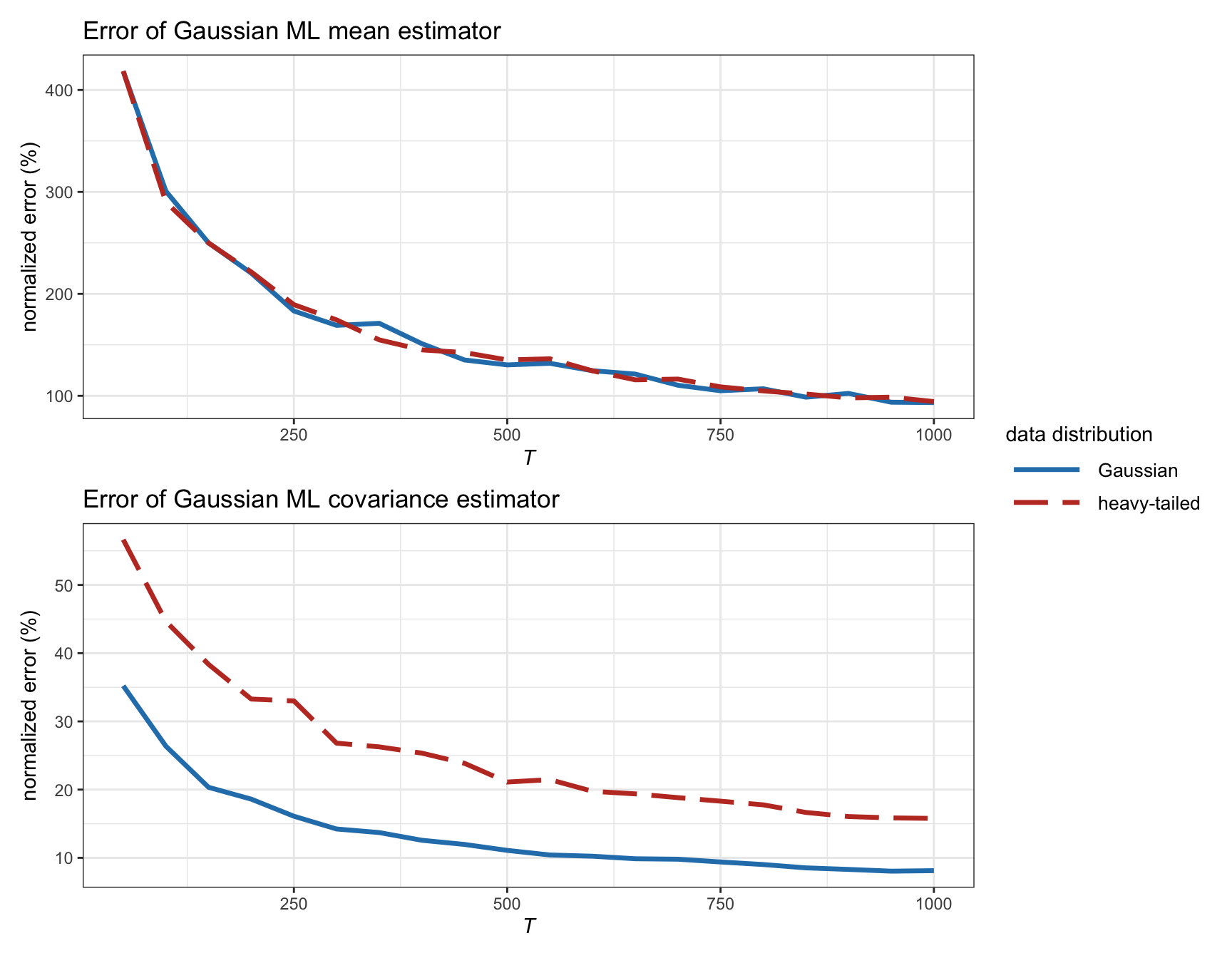
Figure 3.6: Estimation error of Gaussian ML estimators vs. number of observations (with \(N=100\)).
Figure 3.7 examines in more detail the effect of the heavy tails in the estimation error for synthetic data following a \(t\) distribution with degrees of freedom \(\nu\). We can confirm that the error in the estimation of the mean remains the same, whereas the estimation of the covariance matrix becomes worse as the distribution exhibits heavier tails. Nevertheless, we should not forget that the size of the error is one order of magnitude larger for the mean than for the covariance matrix.
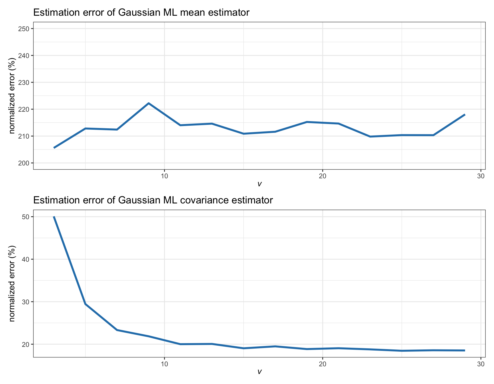
Figure 3.7: Estimation error of Gaussian ML estimators vs. degrees of freedom in a \(t\) distribution (with \(T=200\) and \(N=100\)).
References
To be precise, the term \(f(\bm{x}_0)d\bm{x}\) gives the probability of observing \(\bm{x}\) in a region centered around \(\bm{x}_0\) with volume \(d\bm{x}\).↩︎