\( \newcommand{\bm}[1]{\boldsymbol{#1}} \newcommand{\textm}[1]{\textsf{#1}} \def\T{{\mkern-2mu\raise-1mu\mathsf{T}}} \newcommand{\R}{\mathbb{R}} % real numbers \newcommand{\E}{{\rm I\kern-.2em E}} \newcommand{\w}{\bm{w}} % bold w \newcommand{\bmu}{\bm{\mu}} % bold mu \newcommand{\bSigma}{\bm{\Sigma}} % bold mu \newcommand{\bigO}{O} %\mathcal{O} \renewcommand{\d}[1]{\operatorname{d}\!{#1}} \)

12.2 Hierarchical clustering and dendrograms

Clustering is a multivariate statistical data analysis used in many fields, including machine learning, data mining, pattern recognition, bioinformatics, and financial markets. It is an unsupervised classification method that groups elements into clusters of similar characteristics based on the data.

Hierarchical clustering refers to the formation of a recursive nested clustering. It builds a binary tree of data points that represents nested groups of similar points based on a measure of distance. On the other hand, partitional clustering finds all the clusters simultaneously as a partition of the data points without imposing any hierarchical structure. One benefit of hierarchical clustering is that it allows exploring data on different levels of granularity.

A dendrogram is simply a visual representation of such a tree that encodes the successive or hierarchical clustering. It provides a highly interpretable complete description of the hierarchical clustering in a graphical format. This is one of the main reasons for the popularity of hierarchical clustering methods. For instance, in Example 12.1, items #1 and #2 have the smallest distance of \(0.5659\) and would be clustered together first, followed by item #3. This is illustrated in the dendrogram in Figure 12.1, which shows in a tree structure this bottom-up hierarchical clustering process.

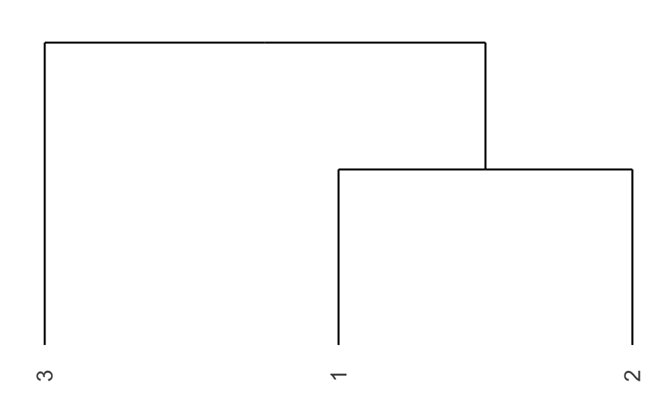
Figure 12.1: Dendrogram of toy Example 12.1.

Basic procedure

Hierarchical clustering requires a distance matrix \(\bm{D}\) and proceeds to sequentially cluster items based on distance (Hastie et al., 2009; G. James et al., 2013). Strategies for hierarchical clustering can be divided into two basic paradigms: agglomerative (bottom-up) and divisive (top-down). Bottom-up strategies start with every item representing a singleton cluster and then combine the clusters sequentially, reducing the number of clusters at each step until only one cluster is left. Alternatively, top-down strategies start with all the items in one cluster and recursively divide each cluster into smaller clusters. Each level of the hierarchy represents a particular grouping of the data into disjoint clusters of observations. The entire hierarchy represents an ordered sequence of such groupings.

Consider the bottom-up approach in which, at each step, the two closest (least dissimilar) clusters are merged into a single cluster, producing one less cluster at the next higher level. This process requires a measure of dissimilarity between two clusters and different definitions of the distance between clusters can produce radically different dendrograms. In addition, there are different ways to merge the clusters, termed linkage clustering; most notably:⁵⁵

• single linkage: the distance between two clusters is the minimum distance between any two points in the clusters, which is related to the so-called minimum spanning tree (MST);

• complete linkage: the distance between two clusters is the maximum of the distance between any two points in the clusters;

• average linkage: the distance between two clusters is the average of the distance between any two points in the clusters; and

• Ward’s method: the distance between two clusters is the increase of the squared error from when two clusters are merged, which is related to distances between centroids of clusters (Ward, 1963).

The effect of the linkage clustering method is very important as it significantly affects the obtained hierarchical clustering (Raffinot, 2018a). The single linkage tends to produce a “chaining” effect in the tree (described later in Section 12.3.1) and an imbalance of large and small groups, whereas the complete linkage typically produces more balanced groups, and the average linkage is an intermediate case. Ward’s method often produces similar results to the average linkage. Figure 12.2 shows the dendrograms corresponding to the four different linkage methods for some S&P 500 stocks corresponding to different sectors during 2015-2020. Various numbers of clusters can be achieved by cutting the tree at distinct heights; for instance, four clusters can be acquired through suitable cuts, although they differ depending on the linkage methods used.

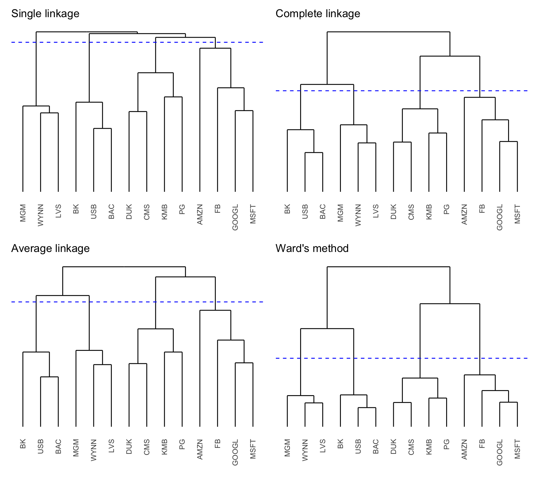
Figure 12.2: Dendrograms of S&P 500 stocks (with cut to produce four clusters).

Number of clusters

Traversing the dendrogram top-down, one starts with a giant cluster containing all the items all the way down to \(N\) singleton clusters, each containing a single item. In practice, however, it may not be necessary or convenient to deal with \(N\) singleton clusters, in order to avoid overfitting of the data.

Representing the data by fewer clusters necessarily loses certain fine details, but achieves simplification. However, choosing the best number of clusters is not easy: too few clusters and the algorithm may fail to find true patterns; too many clusters and it may discover spurious patterns that do not really exist. Thus, it is convenient to have an automatic way of detecting the most appropriate number of clusters to avoid overfitting.

One popular way to determine the number of clusters is the so-called gap statistic (Tibshirani et al., 2001). Basically, it compares the logarithm of the empirical within-cluster dissimilarity and the corresponding one for uniformly distributed data, which is a distribution with no obvious clustering.

Quasi-diagonalization of correlation matrix

The hierarchical clustering can be used to reorder the items in the correlation matrix so that similar assets (i.e., items that cluster early) are placed closer to each other, whereas dissimilar assets are placed far apart. This is called matrix seriation or matrix quasi-diagonalization and it is a very old statistical technique used to rearrange the data to show the inherent clusters clearly. This rearranges the original correlation matrix of assets into a quasi-diagonal correlation matrix, revealing similar assets as blocks along the main diagonal, whereas the correlation matrix of the original randomly ordered items presents no visual pattern.

To illustrate this process, Figure 12.3 shows the heatmaps of the original correlation matrix (with randomly ordered stocks) and the quasi-diagonal version (i.e., after a reordering of the stocks to visualize better the correlated stocks along the diagonal blocks) based on the hierarchical clustering (using single linkage). From the quasi-digonal correlation matrix one can clearly identify four clusters, which can also be observed in the dendrograms in Figure 12.2.

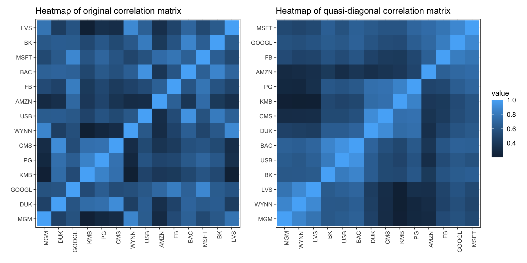
Figure 12.3: Effect of seriation in the correlation matrix of S&P 500 stocks.

References

Hastie, T., Tibshirani, R., and Friedman, J. (2009). The elements of statistical learning. Springer.

James, G., Witten, D., Hastie, T., and Tibshirani, R. (2013). An introduction to statistical learning: With applications in R. Springer.

Raffinot, T. (2018a). Hierarchical clustering-based asset allocation. The Journal of Portfolio Management, 44(2), 89–99.

Tibshirani, R., Walther, G., and Hastie, T. (2001). Estimating the number of clusters in a data set via the gap statistic. Journal of the Royal Statistical Society. Series B: Statistical Methodology, 63(2), 411–423.

Ward, J. H. (1963). Hierarchical grouping to optimize an objective function. Journal of the American Statistical Association, 58(301), 236–244.

---

55. Hierarchical clustering is a fundamental method available in most programming languages; for example, the base function hclust() in R and the method scipy.cluster.hierarchy.linkage() from the Python library scipy.↩︎