B.7 Majorization–Minimization (MM)
The majorization–minimization (MM) method (or framework) approximates a difficult optimization problem by a sequence of simpler problems. We now give a brief description. For details, the reader is referred to the concise tutorial in Hunter and Lange (2004), the long tutorial with applications in Y. Sun et al. (2017), and the convergence analysis in Razaviyayn et al. (2013).
Suppose the following (difficult) problem is to be solved: \[\begin{equation} \begin{array}{ll} \underset{\bm{x}}{\textm{minimize}} & f(\bm{x})\\ \textm{subject to} & \bm{x} \in \mathcal{X}, \end{array} \tag{B.12} \end{equation}\] where \(f\) is the (possibly nonconvex) objective function and \(\mathcal{X}\) is a (possibly nonconvex) set. Instead of attempting to directly obtain a solution \(\bm{x}^\star\) (either a local or a global solution), the MM method will produce a sequence of iterates \(\bm{x}^0, \bm{x}^1, \bm{x}^2,\dots\) that will converge to \(\bm{x}^\star\).
More specifically, at iteration \(k\), MM approximates the objective function \(f(\bm{x})\) by a surrogate function around the current point \(\bm{x}^k\), denoted by \(u\left(\bm{x};\bm{x}^k\right)\), leading to the sequence of (simpler) problems: \[ \bm{x}^{k+1}=\underset{\bm{x}\in\mathcal{X}}{\textm{arg min}}\;u\left(\bm{x};\bm{x}^k\right), \qquad k=0,1,2,\dots \] This iterative process is illustrated in Figure B.6.

Figure B.6: Illustration of sequence of surrogate problems in MM.
In order to guarantee convergence of the iterates, the surrogate function \(u\left(\bm{x};\bm{x}^k\right)\) has to satisfy the following technical conditions (Razaviyayn et al., 2013; Y. Sun et al., 2017):
- upper-bound property: \(u\left(\bm{x};\bm{x}^k\right) \geq f\left(\bm{x}\right)\);
- touching property: \(u\left(\bm{x}^k;\bm{x}^k\right) = f\left(\bm{x}^k\right)\); and
- tangent property: \(u\left(\bm{x};\bm{x}^k\right)\) must be differentiable with \(\nabla u\left(\bm{x};\bm{x}^k\right) = \nabla f\left(\bm{x}\right)\).
One immediate consequence of the first two conditions is the monotonicity property of MM, that is, \(f\left(\bm{x}^{k+1}\right) \leq f\left(\bm{x}^k\right),\) while the third condition is necessary for the convergence of the iterates \(\bm{x}^0, \bm{x}^1, \bm{x}^2,\dots\) – the third condition can be relaxed by requiring continuity and directional derivatives instead (Razaviyayn et al., 2013; Y. Sun et al., 2017). More specifically, under the above technical conditions, if the feasible set \(\mathcal{X}\) is convex, then every limit point of the sequence \(\{\bm{x}^k\}\) is a stationary point of the original problem (Razaviyayn et al., 2013).
The surrogate function \(u\left(\bm{x};\bm{x}^k\right)\) is also referred to as the majorizer because it is an upper bound on the original function. The fact that, at each iteration, first the majorizer is constructed and then it is minimized gives the name majorization–minimization to the method.
In practice, the difficulty lies in finding the appropriate majorizer \(u\left(\bm{x};\bm{x}^k\right)\) that satisfies the technical conditions for convergence and, at the same time, leads to a simpler easy-to-solve surrogate problem. The reader is referred to Y. Sun et al. (2017) for techniques and examples on majorizer construction. Once the majorizer has been chosen, the MM description is very simple, as summarized in Algorithm B.7.
Algorithm B.7: MM to solve the general problem in (B.12).
Choose initial point \(\bm{x}^0\in\mathcal{X}\);
Set \(k \gets 0\);
repeat
- Construct majorizer of \(f(\bm{x})\) around current point \(\bm{x}^k\) as \(u\left(\bm{x};\bm{x}^k\right)\);
- Obtain next iterate by solving the majorized problem: \[\bm{x}^{k+1}=\underset{\bm{x}\in\mathcal{X}}{\textm{arg min}}\;u\left(\bm{x};\bm{x}^k\right);\]
- \(k \gets k+1\);
until convergence;
B.7.1 Convergence
MM is an extremely versatile framework for deriving practical algorithms. In addition, there are theoretical guarantees for convergence (Razaviyayn et al., 2013; Y. Sun et al., 2017) as summarized in Theorem B.4.
Theorem B.4 (Convergence of MM) Suppose that the majorizer \(u\left(\bm{x};\bm{x}^k\right)\) satisfies the previous technical conditions and the feasible set \(\mathcal{X}\) is convex. Then, every limit point of the sequence \(\{\bm{x}^k\}\) is a stationary point of the original problem.
For nonconvex \(\mathcal{X}\), convergence must be evaluated on a case-by-case basis – for examples, refer to J. Song et al. (2015), Y. Sun et al. (2017), Kumar et al. (2019), and Kumar et al. (2020).
B.7.2 Accelerated MM
Unfortunately, in some situations MM may require many iterations to convergence. This may happen if the surrogate function \(u\left(\bm{x};\bm{x}^k\right)\) is not tight enough due to the strict global upper-bound requirement. For that reason, it is necessary to resort to some acceleration techniques.
One popular quasi-Newton acceleration technique that works well in practice is the so-called SQUAREM (Varadhan and Roland, 2008). Denote the standard MM update as \[ \bm{x}^{k+1} = \textm{MM}(\bm{x}^k), \] where \[ \textm{MM}(\bm{x}^k) \triangleq \underset{\bm{x}\in\mathcal{X}}{\textm{arg min}}\;u\left(\bm{x};\bm{x}^k\right). \] Accelerated MM takes two standard MM steps and combines them in a sophisticated way, with a final third step to guarantee feasibility. The details are as follows: \[ \begin{aligned} \textm{difference first update:} \qquad \bm{r}^k &= R(\bm{x}^k) \triangleq \textm{MM}(\bm{x}^k) - \bm{x}^k;\\ \textm{difference of differences:} \qquad \bm{v}^k &= R(\textm{MM}(\bm{x}^k)) - R(\bm{x}^k);\\ \textm{stepsize:} \qquad \alpha^k &= -\textm{max}\left(1, \|\bm{r}^k\|_2/\|\bm{v}^k\|_2\right);\\ \textm{actual step taken:} \qquad \bm{y}^k &= \bm{x}^k - \alpha^k \bm{r}^k;\\ \textm{final update on actual step:} \quad \bm{x}^{k+1} &= \textm{MM}(\bm{y}^k). \end{aligned} \] The last step, \(\bm{x}^{k+1}=\textm{MM}(\bm{y}^k)\), can be eliminated (to avoid having to solve the majorized problem a third time) if we can make sure \(\bm{y}^k\) is feasible, becoming \(\bm{x}^{k+1}=\bm{y}^k.\)
B.7.3 Illustrative Examples
We now examine a few illustrative examples of application of MM, along with numerical experiments.
Example B.7 (Nonnegative LS via MM) Consider the nonnegative least-squares problem \[ \begin{array}{ll} \underset{\bm{x}\geq\bm{0}}{\textm{minimize}} & \frac{1}{2}\left\Vert \bm{A}\bm{x}-\bm{b}\right\Vert^2_{2}, \end{array} \] where \(\bm{b}\in\R^{m}_{+}\) has nonnegative elements and \(\bm{A}\in\R^{m\times n}_{++}\) has positive elements.
Due to the nonnegativity constraints, we cannot use the conventional LS closed-form solution \(\bm{x}^{\star}=(\bm{A}^\T\bm{A})^{-1}\bm{A}^\T\bm{b}\). Since the problem is a QP, we can then resort to using a QP solver. More interestingly, we can develop a simple iterative algorithm based on MM.
The critical step in MM is to find the appropriate majorizer. In this case, one convenient majorizer of the function \(f(\bm{x}) = \frac{1}{2}\left\Vert \bm{A}\bm{x}-\bm{b}\right\Vert^2_{2}\) is \[ u\left(\bm{x};\bm{x}^k\right) = f\left(\bm{x}^k\right) + \nabla f\left(\bm{x}^k\right)^\T \left(\bm{x} - \bm{x}^k\right) + \frac{1}{2} \left(\bm{x} - \bm{x}^k\right)^\T \bm{\Phi}\left(\bm{x}^k\right) \left(\bm{x} - \bm{x}^k\right), \] where \(\nabla f\left(\bm{x}^k\right) = \bm{A}^\T\bm{A}\bm{x}^k - \bm{A}^\T\bm{b}\) and \(\bm{\Phi}\left(\bm{x}^k\right) = \textm{Diag}\left(\frac{\left[\bm{A}^\T\bm{A}\bm{x}^k\right]_1}{x_1^k},\dots,\frac{\left[\bm{A}^\T\bm{A}\bm{x}^k\right]_n}{x_n^k}\right)\). It can be verified that \(u\left(\bm{x};\bm{x}^k\right)\) is a valid majorizer because (i) \(u\left(\bm{x};\bm{x}^k\right) \geq f\left(\bm{x}\right)\) (which can be proved using Jensen’s inequality), (ii) \(u\left(\bm{x}^k;\bm{x}^k\right) = f\left(\bm{x}^k\right)\), and (iii) \(\nabla u\left(\bm{x}^k;\bm{x}^k\right) = \nabla f\left(\bm{x}^k\right).\)
Therefore, the sequence of majorized problems to be solved for \(k=0,1,2,\dots\) is \[ \begin{array}{ll} \underset{\bm{x}\geq\bm{0}}{\textm{minimize}} & \nabla f\left(\bm{x}^k\right)^\T \bm{x} + \frac{1}{2} \left(\bm{x} - \bm{x}^k\right)^\T \bm{\Phi}\left(\bm{x}^k\right) \left(\bm{x} - \bm{x}^k\right), \end{array} \] with solution \(\bm{x} = \bm{x}^k - \bm{\Phi}\left(\bm{x}^k)^{-1}\nabla f\;(\bm{x}^k\right).\)
This finally leads to the following MM iterative algorithm: \[ \bm{x}^{k+1} = \bm{c}^k \odot \bm{x}^k, \qquad k=0,1,2,\dots \] where \(c_i^k = \frac{[\bm{A}^\T\bm{b}]_i}{[\bm{A}^\T\bm{A}\bm{x}^k]_i}\) and \(\odot\) denotes elementwise product. Figure B.7 shows the convergence of the MM iterates.
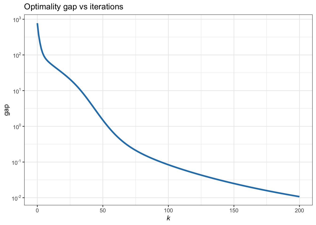
Figure B.7: Convergence of MM for the nonnegative LS.
Example B.8 (Reweighted LS for \(\ell_1\)-norm minimization via MM) Consider the \(\ell_1\)-norm minimization problem \[ \begin{array}{ll} \underset{\bm{x}}{\textm{minimize}} & \left\Vert \bm{A}\bm{x} - \bm{b}\right\Vert_1. \end{array} \]
If instead we had the \(\ell_2\)-norm in the formulation, then we would have the conventional LS solution \(\bm{x}^{\star}=(\bm{A}^\T\bm{A})^{-1}\bm{A}^\T\bm{b}\). In any case, this problem is an LP and can be solved with an LP solver. However, we can develop a simple iterative algorithm based on MM that leverages the closed-form LS solution.
The critical step in MM is to find the appropriate majorizer. In this case, since we would like to use the LS solution, we want the majorizer to have the form of an LS problem, that is, we want to go from \(\|\cdot\|_1\) to \(\|\cdot\|_2^2\). This can be achieved if we manage to majorize \(|t|\) in terms of \(t^2\). Indeed, a quadratic majorizer for \(f(t)=|t|\) (for simplicitly we assume \(t\neq0\)) is (Y. Sun et al., 2017) \[ u(t;t^k) = \frac{1}{2|t^k|}\left(t^2 + (t^k)^2\right). \] Consequently, a majorizer of the function \(f(\bm{x}) = \left\Vert \bm{A}\bm{x} - \bm{b}\right\Vert_1\) is \[ u\left(\bm{x};\bm{x}^k\right) = \sum_{i=1}^n \frac{1}{2\left|[\bm{A}\bm{x}^k - \bm{b}]_i\right|} \left([\bm{A}\bm{x} - \bm{b}]_i^2 - [\bm{A}\bm{x}^k - \bm{b}]_i^2 \right). \]
Therefore, the sequence of majorized problems to be solved for \(k=0,1,2,\dots\) is \[ \begin{array}{ll} \underset{\bm{x}}{\textm{minimize}} & \left\|(\bm{A}\bm{x} - \bm{b}) \odot \bm{c}^k\right\|_2^2, \end{array} \] where \(c_i^k = \sqrt{\frac{1}{2\left|[\bm{A}\bm{x}^k - \bm{b}]_i\right|}}\).
This finally leads to the following MM iterative algorithm: \[ \bm{x}^{k+1}=(\bm{A}^\T\textm{Diag}^2(\bm{c}^k)\bm{A})^{-1}\bm{A}^\T\textm{Diag}^2(\bm{c}^k)\bm{b}, \qquad k=0,1,2,\dots \] Figure B.8 shows the convergence of the MM iterates.
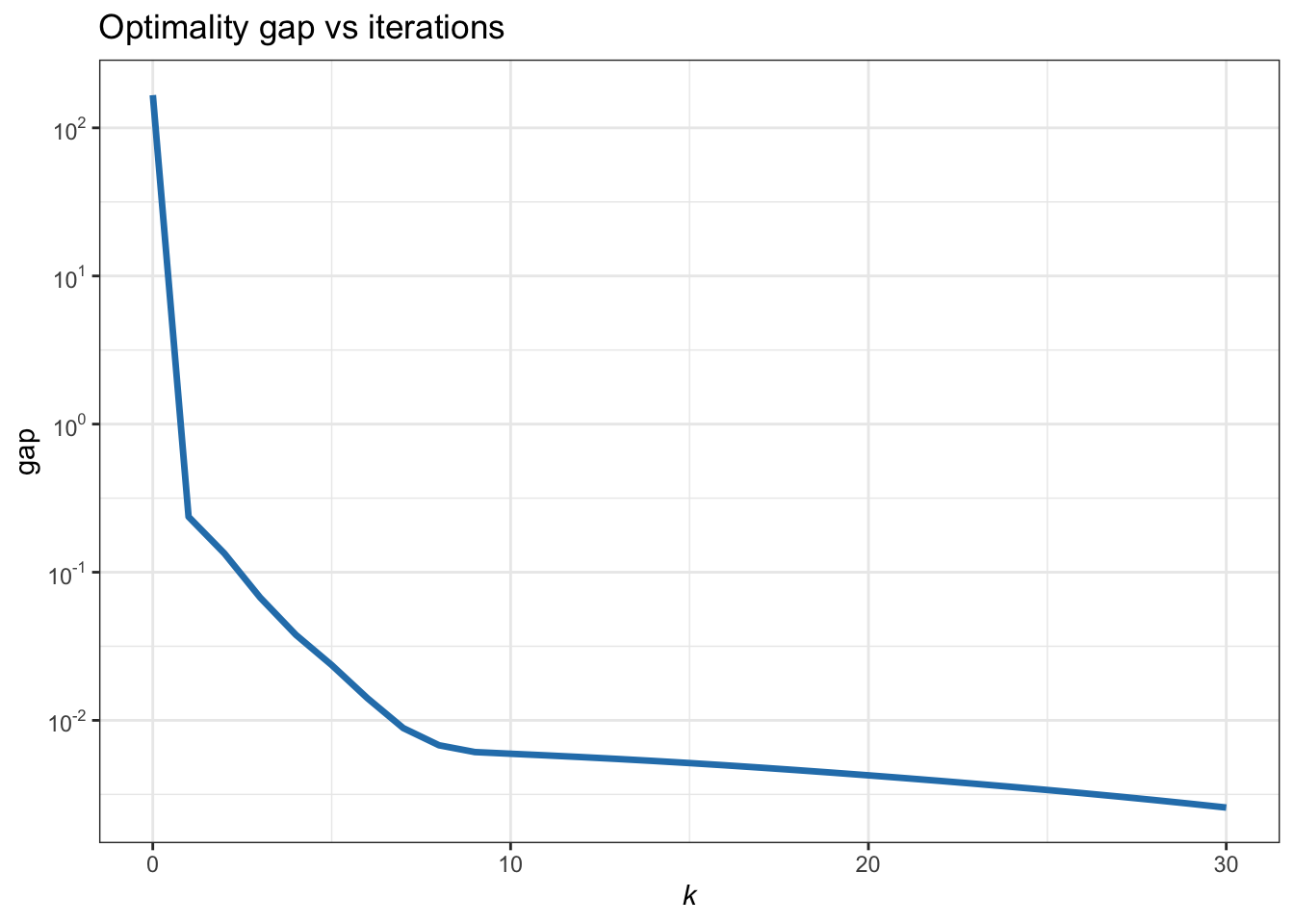
Figure B.8: Convergence of MM for the \(\ell_1\)-norm minimization (reweighted LS).
Example B.9 (\(\ell_2\)–\(\ell_1\)-norm minimization via MM) Consider the \(\ell_2\)–\(\ell_1\)-norm minimization problem \[ \begin{array}{ll} \underset{\bm{x}}{\textm{minimize}} & \frac{1}{2}\|\bm{A}\bm{x} - \bm{b}\|_2^2 + \lambda\|\bm{x}\|_1. \end{array} \]
This problem can be conveniently solved via BCD (see Section B.6), via SCA (see later Section B.8), or simply by calling a QP solver. Interestingly, we can develop a simple iterative algorithm based on MM that leverages the element-by-element closed-form solution (Zibulevsky and Elad, 2010).
In this case, one possible majorizer of the objective function \(f(\bm{x})\) is \[ u\left(\bm{x};\bm{x}^k\right) = \frac{\kappa}2{}\|\bm{x} - \bm{\bar{x}}^k\|_2^2 + \lambda\|\bm{x}\|_1 + \textm{constant}, \] where \(\bm{\bar{x}}^k = \bm{x}^k - \frac{1}{\kappa}\bm{A}^\T\left(\bm{A}\bm{x}^k - \bm{b}\right)\). The way to verify that it is indeed a majorizer of \(f(\bm{x})\) is by writing it as \[ u\left(\bm{x};\bm{x}^k\right) = f(\bm{x}) + \textm{dist}\left(\bm{x}, \bm{x}^k\right), \] where \(\textm{dist}\left(\bm{x}, \bm{x}^k\right) = \frac{\kappa}{2}\|\bm{x} - \bm{x}^k\|_2^2 - \frac{1}{2}\|\bm{A}\bm{x} - \bm{A}\bm{x}^k\|_2^2\) is a distance measure with \(\kappa > \lambda_\textm{max}\left(\bm{A}^\T\bm{A}\right)\).
Therefore, the sequence of majorized problems to be solved for \(k=0,1,2,\dots\) is \[ \begin{array}{ll} \underset{\bm{x}}{\textm{minimize}} & \frac{\kappa}{2}\left\|\bm{x} - \bm{\bar{x}}^k\right\|_2^2 + \lambda\|\bm{x}\|_1, \end{array} \] which decouples into each component of \(\bm{x}\) with closed-form solution given by the soft-thresholding operator (see Section B.6).
This finally leads to the following MM iterative algorithm: \[ \bm{x}^{k+1} = \mathcal{S}_{\lambda/\kappa} \left(\bm{\bar{x}}^k\right), \qquad k=0,1,2,\dots, \] where \(\mathcal{S}_{\lambda/\kappa}(\cdot)\) is the soft-thresholding operator defined in (B.11). Figure B.9 shows the convergence of the MM iterates.
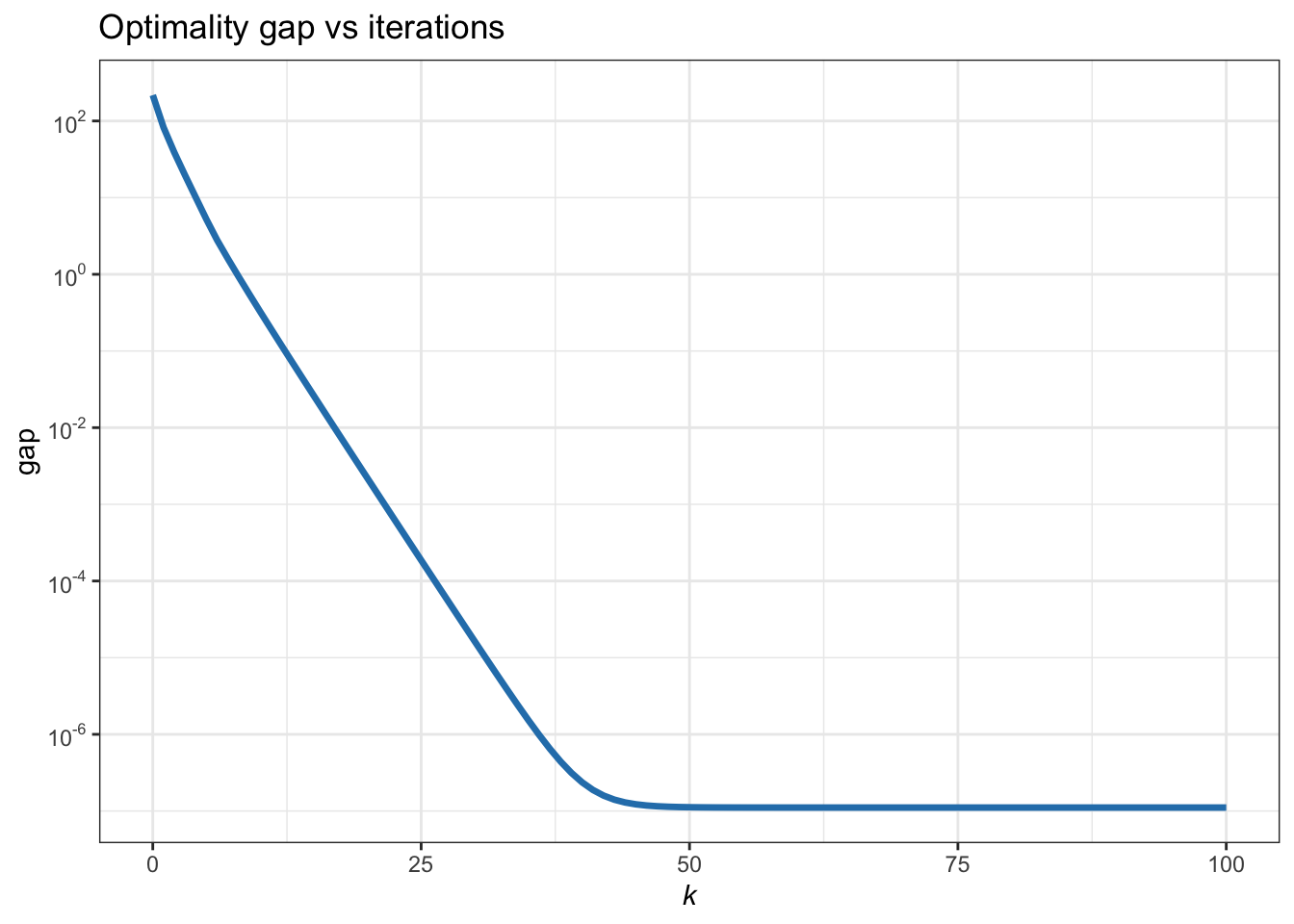
Figure B.9: Convergence of MM for the \(\ell_2\)–\(\ell_1\)-norm minimization.
B.7.4 Block MM
Block MM is a combination of BCD and MM. Suppose that not only is the original problem (B.12) difficult to solve directly, but also a direct application of MM is still too difficult. If the variables can be partitioned into \(n\) blocks \(\bm{x} = (\bm{x}_1,\dots,\bm{x}_n)\) that are separately constrained, \[ \begin{array}{ll} \underset{\bm{x}}{\textm{minimize}} & f(\bm{x}_1,\dots,\bm{x}_n)\\ \textm{subject to} & \bm{x}_i \in \mathcal{X}_i, \qquad i=1,\dots,n, \end{array} \] then we can successfully combine BCD and MM. The idea is to solve block by block as in BCD (see Section B.6) but majorizing each block \(f(\bm{x}_i)\) with \(u\left(\bm{x}_i;\bm{x}^k\right)\) (Razaviyayn et al., 2013; Y. Sun et al., 2017).